Two ways to write autologistic multistate occupancy models in `JAGS`
This is the second post in a series I am writing on multistate occupancy models. I will be building off my previous example of a static multistate model, so if you’ve not read the first post be sure to check it out here. Likewise, if want more of an introduction to autologistic occupancy models, please see this post here.
Before I jump into things, let me remind you what multistate and autologistic occupancy models are. Multistate occupancy models partition the probability of success (i.e., species presence) into multiple discrete states. In my previous example, we estimated the probability of three states:
- That owls were not present
- That owls were present but not breeding
- That owls were present and breeding.
Autologistic occupancy models, on the other hand, are a simplified version of a dynamic occupancy model that estimates species occupancy instead of local colonization / extinction dynamics. They include an additional term in their logit-linear predictor to account for temporal dependence between primary sampling periods.
Therefore, an autologistic multistate model estimates multiple discrete states across space and through time, and includes additional parameters to account for temporal dependence (e.g., a site where we found owls breeding at time t-1 may be more likely to have owls that breed there at time t). To my knowledge, this class of model has never received a formal write-up, and so it has rarely been used in the literature. Nevertheless, it is a very useful model to know if you are interested in applying a multistate model to data over time.
In this post I will explain two different ways to write a three state model for a single species. The first model is the simplest parameterization, and uses the logit-link to estimate the occupancy probability of multiple states. I like this model for two reasons. First, it uses a standard link function that people should be familiar with, which makes it more approachable. Second, it is the absolute simplest parameterization of an autologistic multistate model, and so may be your best bet if you have a small sample size. In the second formulation, I use the softmax function to parameterize the model and include extra autologistic terms to estimate turnover among states over time. For example, if a site was in state 2 (owls present, not breeding) at time t-1, the probability it transitions to state 3 (owls present & breeding) at time t may be different than a site in state 3 that remains in state 3 from one time period to the next. This second model is useful for two reasons. First, the way this model is parameterized is very similar to multistate occupancy models for potentially interacting species. Therefore, understanding how this model works here will hopefully help you better understand how the Rota et al. (2016) or Fidino et al. (2018) models work. Second, it demonstrates that you have multiple choices to make when you attempt to use such a model, and so it’s important to critically think about what it is you are interested in estimating (and whether or not you may have the sample size to do so).
Again, we are going to continue with the example of modeling the distribution of great horned owls and their breeding territory, except we now have data over time as well. Therefore, assume we have conducted j in 1,…,J surveys at s in 1,…,S sites throughout Chicago, Illinois during t in 1,…,T great horned owl breeding seasons. During each of these surveys we can record 1 of 3 possible values:
- No detection of an owl
- Detection of an adult owl but no detection of a young owl
- Detection of a young owl (i.e., reproductive success)
We store these observations in a S by J by T array \(\boldsymbol{Y}\). This lets us estimate three separate states: owls are not present (state = 1), owls are present but not breeding (state = 2), and owls are present and breeding (state = 3). However, the probability of occupancy of the different states at site s and time t is going to depend on the the state at time t-1. Therefore, instead of having a vector of occupancy probabilties, we place them in a transition probability matrix (TPM), which stores the probability of transitioning from one state to another in a single time unit:
\[\boldsymbol{\psi_{s,t}} = \begin{bmatrix} \psi_{s,t}^1 & \psi_{s,t}^{2} & \psi_{s,t}^3 \\ \psi_{s,t}^{1|2} & \psi_{s,t}^{2|2} & \psi_{s,t}^{3|2} \\ \psi_{s,t}^{1|3} & \psi_{s,t}^{2|3} & \psi_{s,t}^{3|3} \end{bmatrix}\]One important aspect to remember about TPMs is that one dimension of the matrix represents “from this state” and the other dimension represents “to that state”. In our case, the rows are the former and the columns are the latter. Because of this, each row of our TPM sums to 1. For example, to locate the transition probability from state 3 to state 2, we need to look for the element in row 3 (“from” state 3) and column 2 (“to” state 2), which is \(\psi_{s,t}^{2|3}\). I’ve added the conditional probabilities (e.g,. 2|3) on the 2nd and 3rd rows to remind you that we are including autologistic terms to help account for temporal dependence between time units.
Before I break down how TPMs apply to autologistic occupancy models, however, I want to acknowledge that interpreting TPMs can be difficult, and this may be the first time you have heard about them. As such, I’m going to work through a simple example of a TPM, explain some important qualities that they have, and introduce you to the markovchain package in R, which has some useful functions for dealing with TPMs.
Links to different parts of this post
- The transition probability matrix. What is how and how to use it.
- An autologistic multistate occupancy model that uses the logit link
- The logit-link model written in JAGS
- Simulating some data and plotting the results from the logit-link model
- An autologistic multistate model occupancy that uses the softmax function
- The softmax model written in JAGS
- Simulating some data and plotting the results from the softmax model
The transition probability matrix. What it is and how to use it.
Imagine we have this TPM:
\[TPM = \begin{bmatrix} 0.3 & 0.4 & 0.3 \\ 0.6 & 0.2 & 0.2 \\ 0.1 & 0.5 & 0.4 \end{bmatrix}\]It has three states, and the probability of transitioning from one state to another in a single time unit varies based on what state you are currently in. Each row of this TPM sums to one. Another feature of this TPM is that it does not have any absorbing states (i.e., a state that, once entered, cannot be left). Because of this, this TPM is an irreducible stochastic matrix, which has some pretty unique properties. Perhaps the most useful in our case is that you can estimate a stationary probability vector, \(\boldsymbol{\pi}\), which describes the long-term distribution of the TPM (i.e., the expected proportion of time each state should be visited). In terms of autologistic multistate occupancy models, this stationary probability vector describes the expected occupancy of each of the three states!
How do you calculate \(\boldsymbol{\pi}\)? You need to solve this equation:
\[\boldsymbol{\pi}TPM = \boldsymbol{\pi}\]This equation, as it turns out, looks almost identical to the equation for left eigenvectors:
\[x A = \lambda x\]where x, our left eigenvector, is a non-zero row vector that satisfies the equation above, A is a n by n matrix (the TPM), and \(\lambda\) is an eigenvalue, which is a special scalar associated to a system of linear equations that ensures the equality above holds.
A n by n matrix has n eigenvectors and n eigenvalues. However, for our purposes we only need the first of each, which brings me to another unique property of TPMs, the leading eigenvalue of a TPM is always 1. This means that to calculate the left eigenvectors for a TPM we don’t need to worry about the eigenvalue \(\lambda\). Therefore, we can simplify the equation for left eigenvectors so that it is equivalent the first equation I shared in this section (just with different symbols).
\[\begin{eqnarray} x A &=& \lambda x \nonumber \\ x A &=& x\nonumber \\ \boldsymbol{\pi}TPM &=& \boldsymbol{\pi} \end{eqnarray}\]Here is how we can do this in R:
# Our TPM
tpm <- matrix(
  c(0.3,0.4,0.3,
    0.6,0.2,0.2,
    0.1,0.5,0.4),
  ncol = 3,
  nrow = 3,
  byrow = TRUE
)

# base::eigen() gives right eigenvectors, which satisfy the equation
#   A %*% x = lambda %*%x (which is not the equation we are trying
#   to solve). However, we can invert the right eigenvector matrix to
#   get our left eigenvectors. The output of this function is a named list
#  with (eigen)'values' and (eigen)'vectors'.
right <- eigen(tpm)

# See that the first eigenvalue of our TPM is 1
round(right$values,2)

[1]  1.00 -0.16  0.06

# Calculate the generalized inverse of the right eigenvectors
#  to get the left eigenvectors
left_vectors <- MASS::ginv(right$vectors)

# Check really quickly that the decomposition of our
#  matrix is correct, this should return the tpm (it does).
right$vectors%*%diag(right$values)%*%left_vectors

     [,1] [,2] [,3]
[1,]  0.3  0.4  0.3
[2,]  0.6  0.2  0.2
[3,]  0.1  0.5  0.4

# All we need to do is normalize the first row of
#   the left eigenvectors (i.e., divide each value
#   by the sum of the first row). To get the
#   stationary distribution.
stationary_dist <- left_vectors[1,]/sum(left_vectors[1,])

# Check out the stationary distribution,
#   in this case the amount of time spent in
#   each state is about 0.33.
stationary_dist
[1] 0.3486239 0.3577982 0.2935780

# These values fulfill the equation pi %*% tpm = pi
as.numeric(stationary_dist %*% tpm)
[1] 0.3486239 0.3577982 0.2935780
Now, you can write a function to do this for you if you’d like, but you can also get the stationary distribution using markovchain::SteadyStates() just as easily.
library(markovchain)

# Our TPM
tpm <- matrix(
  c(0.3,0.4,0.3,
    0.6,0.2,0.2,
    0.1,0.5,0.4),
  ncol = 3,
  nrow = 3,
  byrow = TRUE
)
# Make tpm a markovchain
markov_tpm <- new(
  "markovchain",
  states = c("a", "b", "c"),
  transitionMatrix = tpm,
  byrow = TRUE
)
# The stationary distribution from the markovchain package
stationary_distmc <- markovchain::steadyStates(markov_tpm)

# our stationary distribution from "scratch"
stationary_dist
[1]  0.3486239 0.3577982 0.293578

# our stationary distribution from markovchain package
#   They are equal.
stationary_distmc
             a         b        c
[1,] 0.3486239 0.3577982 0.293578
There are two reasons I took the time to introduce TPMs. First, we are going to use TPMs in our autologistic occupancy model, and because of this we will want to derive the expected occupancy of each state based on the estimated TPM. Likewise, as we will include spatial covariates in this model, our TPM will also spatially vary (i.e., we will calculate \(\pi_s\), not \(\pi\)). Therefore we need to derive the stationary distribution along whatever environmental gradient we include if we are interested to plotting out the expected occupancy of different states (which we probably want to do).
Second, you may not have known it. But you may have already used a similar approach while fitting dynamic occupancy models. As a reminder, dynamic occupancy models estimate local colonization (\(\gamma\)) and extinction (\(\epsilon\)) rates, and you can use this equation to calculate the expected occupancy of your species:
\[E(\psi) = \frac{\gamma}{\gamma + \epsilon}\]This equation provides the same solution as our approach above for a 2x2 TPM. Instead of using this equation, we could still use the left eigenvector approach from above.
# colonization
gamma <- 0.8
# extinction
epsilon <- 0.6

# calculate expected occupancy
ex_occ <- gamma / (gamma + epsilon)

# and tack on the complimentary probability,
#  which is the proportion of landscape the
#  species is absent
ex_occ <- c(ex_occ, 1 - ex_occ)

# give names to vector
names(ex_occ) <- c("present", "absent")


# make a tpm for a dynamic
#  occupancy model, each row
#  sums to 1
dynamic_tpm <- matrix(
  c(1 - epsilon, epsilon,
    gamma, 1 - gamma),
  ncol = 2,
  nrow = 2,
  byrow = TRUE
)

# Calculate steady states using the
#  markovchain package
dynamic_tpm <- new(
  "markovchain",
  states = c("present", "absent"),
  transitionMatrix = dynamic_tpm,
  byrow = TRUE
)

ex_occmc <- markovchain::steadyStates(dynamic_tpm)

# compare outputs. From markovchain
ex_occmc
  present    absent
0.5714286 0.4285714

# from gamma / (gamma + epsilon)
ex_occ
  present    absent
0.5714286 0.4285714

# They are the same!
While it’s relatively simple to derive the expected occupancy from a 2x2 TPM (i.e., a dynamic occupancy model), you will need to use the left eigenvector approach when dealing with larger TPMs (which autologistic multistate occupancy models have). As such, this is really helpful to know! Let’s move on to our models now.
An autologistic multistate occupancy model that uses the logit link
All autologistic multistate occupancy models require two components:
- A TPM for the latent state model
- A detection probability matrix for the data model
However, like I demonstrated in the last post on multistate models, there are different ways you can specify the probabilities for each row vector of the latent state TPM. What I did not tell you however, is that the way you write the latent state probabilities has an influence on what link function you will use to convert your linear predictors to probabilities. For this model, let’s assume there is no temporal variation in occupancy (i.e., no temporal covariates), and let the latent state TPM, \(\boldsymbol{\psi_{s}}\), be:
\[\boldsymbol{\psi_{s}} = \begin{bmatrix} 1 - \omega_{s} & \omega_{s} (1 - \delta_{s}) & \omega_{s} \delta_{s} \\ 1 - \omega_s^{2,3|2,3} & \omega_s^{2,3|2,3} (1 - \delta_{s}) & \omega_s^{2,3|2,3} \delta_{s} \\ 1 - \omega_s^{2,3|2,3} & \omega_s^{2,3|2,3} (1 - \delta_{s}^{3|3}) & \omega_s^{2,3|2,3} \delta_{s}^{3|3} \end{bmatrix}\]The probabilities in \(\boldsymbol{\psi_{s}}\) can be defined as:
- \(\omega_{s}\): The probability of occupancy regardless of breeding status.
- \(\delta_s\): The conditional probability of breeding given presence.
- \(\omega_s^{2,3|2,3}\): The conditional probability of occupancy regardless of breeding status given that the species was present in the last time step.
- \(\delta_{s}^{3|3}\): The conditional probability of breeding given the species was present and breeding in the last time step.
For the first time step, we have no knowledge of species presence or breeding status. Because of this, all we need to do is use the first row of \(\boldsymbol{\psi_{s}}\) to estimate the distribution of each state at t=1 such that:
\[z_{s,t=1} \sim \text{Categorical}(\boldsymbol{\psi_{s,1}})\]Where \(z_{s,t}\) is a Categorical random variable that can take a value of either 1, 2, or 3 depending on what state site s is in at time t. Going through the rest of this equation, it’s important to remember that \(\boldsymbol{\psi_{s}}\) is a S x 3 x 3 array. Therefore, that additional indexing of 1 in \(\boldsymbol{\psi_{s,1}}\) indicates that we selected the first row of the that site-specific TPM, which would be:
\[\boldsymbol{\psi_{s,1}} = \begin{bmatrix}(1-\omega_s) & \omega_s(1-\delta_s) & \omega_s\delta_s\end{bmatrix}\]After we estimate occupancy at t=1, we can use the latent state at \(z_{s,t-1}\) to index the appropriate row of \(\boldsymbol{\psi_{s}}\) for time t. Thus for t>1 the model is:
\[z_{s,t} \sim \text{Categorical}(\boldsymbol{\psi_{s,z_{s,t-1}}}), t>1\]So, for example, if \(z_{s,t-1} = 2\), we grab the 2nd row of our TPM for site s.
Now, the way I wrote out the TPM is a little unique. The probability of the two species presence states (i.e., 2 or 3) are the product of two probabilities (e.g., \(\omega_{s} (1 - \delta_{s})\)). This allows each of these probabilities to take any value between 0 and 1, and each row will still sum to 1. Because of this quality, we can use the logit link instead of the softmax function to specify the linear predictors for each probability. Why can we do that? Because the logit link maps a linear predictor back to a probability between 0 and 1. We just need to specify our logit-linear predictors, convert them back to probabilities, and fill in our TPM. So, for n in 1,…,N covariates in the S by N matrix X and r in 1,…,R covariates in the S by R matrix U, the logit-linear predictors of the four unique probabilities in this TPM are
\[\begin{eqnarray} \text{logit}(\omega_s) &=& \boldsymbol{\beta}^{2,3} \boldsymbol{x}_s &=& \beta_1^{2,3} \times x_{s,1} + \cdots + \beta_N^{2,3} \times x_{s,N} \nonumber\\ \text{logit}(\omega_s^{2,3|2,3}) &=& \boldsymbol{\beta}^{2,3} \boldsymbol{x}_s + \theta_1 &=& \beta_1^{2,3} \times x_{s,1} + \cdots + \beta_N^{2,3} \times x_{s,N} + \theta_1 \nonumber \\ \text{logit}(\delta_s) &=& \boldsymbol{\beta}^3 \boldsymbol{u}_s &=& \beta_1^{3} \times u_{s,1} + \cdots + \beta_R^3 \times u_{s,R} \nonumber \\ \text{logit}(\delta_s^{3|3}) &=& \boldsymbol{\beta}^3 \boldsymbol{u}_s + \theta_2 &=& \beta_1^{3} \times u_{s,1} + \cdots + \beta_R^3 \times u_{s,R} + \theta_2 \nonumber \end{eqnarray}\]Where the first column of both X and U is a vector of 1’s to accomodate the model intercepts. I’ve indexed each of the regression coefficients by the states they apply to. For example, \(\boldsymbol{\beta}^{2,3}\) are regression coefficients associated to the probability of presences ignoring breeding status (i.e., states 2 or 3). Conversely, \(\boldsymbol{\beta}^3\) are regression coefficients associated to the conditional probability of breeding given species presence (i.e,. state 3). Looking at the equations above, the only thing that differs between the linear predictors in \(\omega_s\) and \(\omega_s^{2,3|2,3}\) is the latter linear predictor has the autologistic term \(\theta_1\). Likewise, the only thing that differs between the linear predictors in \(\delta_s\) and \(\delta_s^{3|3}\) is the autologistic term \(\theta_2\). Thus, this specification of an autologistic multistate occupancy model adds two parameters to the model in order to account temporal dependence in species presence or breeding status from one time period to the next.
The data model for an autologistic multistate occupancy model is almost identical to a static multistate occupancy model, except it is indexed by sites (s in 1,..,S), surveys (j in 1,…,J), and time periods (t in 1,…,T). Again, we are going to assume there is no temporal variability in this level of the model (i.e, across t), but adding that in is not hard to do. Thus, let the detection matrix of the data model be:
\[\boldsymbol{\eta}_{s,j} = \begin{bmatrix} 1 & 0 & 0 \\ (1 - \rho_{s,j}^{\omega}) & \rho_{s,j}^{\omega} & 0 \\ (1 - \rho_{s,j}^{\omega}) & \rho_{s,j}^{\omega} (1 - \rho_{s,j}^\delta) & \rho_{s,j}^{\omega} \rho_{s,j}^\delta \end{bmatrix}\]and the two detection probabilities in this matrix can be defined as:
- \(\rho_{s,j}^{\omega}\): The probability of detecting the species regardless of breeding status given species presence.
- \(\rho_{s,j}^{\delta}\): The probability of detecting breeding given breeding occurs.
Again, the rows sum to 1 in this matrix. Likewise, the rows correspond to the state site s is in at time t and the columns correspond to the probability of detecting each state given the row. For example, the only state that can be detected if a site is in state 1 (species absence) is state 1. Thus, we can assume our observed data (\(y_{s,j,t}\)) are also a Categorical random variable such that
\[y_{s,j,t} \sim \text{Categorical}(\boldsymbol{\eta}_{s,j,z[s]})\]where the latent state z at time t indexes the appropriate row of the detection probability matrix. And just like with the latent state model, we can use the logit link for the two unique probabilities for v in 1,…,V covariates that vary by site and survey:
\[\begin{eqnarray} \text{logit}(\rho_{s,j}^{\omega}) &=& \boldsymbol{\alpha}^{\omega} \boldsymbol{k}_{s,j} &=& \alpha_1^{\omega} \times k_{s,j,1} + \cdots + \alpha_V^{\omega} \times k_{s,j,V} \nonumber\\ \text{logit}(\rho_{s,j}^{\delta}) &=& \boldsymbol{\alpha}^{\delta} \boldsymbol{k}_{s,j} &=& \alpha_1^{\delta} \times k_{s,j,1} + \cdots + \alpha_V^{\delta} \times k_{s,j,V} \nonumber \end{eqnarray}\]Finally, for the parameter model (the priors) we can give every parameter vague Logistic(0,1) priors.
The logit-link model written in JAGS
The model above, can be written in JAGS like so. This file can also be found on this github repository here in ./JAGS/autologistic_multistate_logit.R
model{
  #
  # THE LATENT STATE MODEL
  #
  for(site in 1:nsite){
    # Set up the logit linear predictors
    #   Note: I am assuming here that while the model is dynamic,
    #   the probabilities do not vary by year (because the logit
    #   linear predictors do not vary through time).
    # LATENT STATE LINEAR PREDICTORS.
    # Probability of either state 2 or 3
    #  given state at year-1 == 1 (or first year).
    logit(omega[site]) <- inprod(
      beta23, x[site,]
    )
    # Conditional probability of state 3
    logit(delta[site]) <- inprod(
      beta3, u[site,]
    )
    # Probability of either state 2 or 3
    #  given state at year-1 != 1
    logit(omega_cond[site]) <- inprod(
      beta23, x[site,]
    ) + theta23
    # Conditional probability of state 3
    #  given state at year-1 = 3.
    logit(delta_cond[site]) <- inprod(
      beta3, u[site,]
    ) + theta3
    # Fill in the transition matrix
    # latent state probabilities given state == 1
    psi[site,1,1] <- 1 - omega[site]
    psi[site,1,2] <- omega[site] * (1-delta[site])
    psi[site,1,3] <- omega[site] * delta[site]
    # latent state probabilities given state == 2
    psi[site,2,1] <- 1 - omega_cond[site]
    psi[site,2,2] <- omega_cond[site] * (1-delta[site])
    psi[site,2,3] <- omega_cond[site] * delta[site]
    # latent state probabilities given state == 3
    psi[site,3,1] <- 1 - omega_cond[site]
    psi[site,3,2] <- omega_cond[site] * (1-delta_cond[site])
    psi[site,3,3] <- omega_cond[site] * delta_cond[site]
    # Estimate latent state year == 1. Setting to first
    #  row of psi because we have no prior knowledge
    #  on state of site before we started sampling.
    z[site,1] ~ dcat(
      psi[site,1,]
    )
    # Do the remaining years. We grab the correct row
    #  of the transition matrix based on the state in the
    #  previous time step.
    for(year in 2:nyear){
      z[site,year] ~ dcat(
        psi[site,z[site,year-1],]
      )
    }
  }
  #
  # THE DATA MODEL
  #
  for(site in 1:nsite){
    for(survey in 1:nsurvey){
      # Set up the logit linear predictors
      #   Note: I am assuming here that while the model is dynamic,
      #   The probabilities do not vary by year (because the logit
      #   linear predictors do not vary through time).
      # Probability of detecting either state 2 or 3
      logit(eta23[site,survey]) <- inprod(
        rho23, k[site,survey,]
      )
      # Probability of detecting state 3 given 2
      logit(eta3[site,survey]) <- inprod(
        rho3, k[site,survey,]
      )
      # Fill in detection probability matrix
      # First row: TS = 1
      eta[site,survey,1,1] <- 1 # -------------------------------------- OS = 1
      eta[site,survey,1,2] <- 0 # -------------------------------------- OS = 2
      eta[site,survey,1,3] <- 0 # -------------------------------------- OS = 3
      # Second row: TS = 2
      eta[site,survey,2,1] <- 1 - eta23[site,survey] # ----------------- OS = 1
      eta[site,survey,2,2] <- eta23[site,survey] # --------------------- OS = 2
      eta[site,survey,2,3] <- 0 # -------------------------------------- OS = 3
      # Third row: TS = 3
      eta[site,survey,3,1] <- 1 - eta23[site,survey] # ----------------- OS = 1
      eta[site,survey,3,2] <- eta23[site,survey]*(1-eta3[site,survey]) # OS = 2
      eta[site,survey,3,3] <- eta23[site,survey]*eta3[site,survey] # --- OS = 3
      for(yr in 1:nyear){
        # Index the appropriate row of eta based on the current latent state.
        # Again, we are assuming there is no variation among years or sampling.
        y[site,survey,yr] ~ dcat(
          eta[site,survey,z[site,yr],]
        )
      }
    }
  }
  #
  # Priors
  #
  # Pr(latent state 2 or 3)
  for(b2 in 1:nbeta23){
    beta23[b2] ~ dlogis(0,1)
  }
  # Pr(latent state 3)
  for(b3 in 1:nbeta3){
    beta3[b3] ~ dlogis(0,1)
  }
  # Autologistic terms
  theta23 ~ dlogis(0,1)
  theta3 ~ dlogis(0,1)
  # Pr(OS = 2 or 3 | TS = 2 or 3)
  for(ts2 in 1:nts2){
    rho23[ts2] ~ dlogis(0,1)
  }
  # Pr(OS = 3 | TS = 3)
  for(ts3 in 1:nts3){
    rho3[ts3] ~ dlogis(0,1)
  }
}
Simulating some data and plotting the results from the logit-link model
For a look at how I simulated all of these data, check out this github repository here. The file to fit the model and plot out the results is ./R/examples/autologistic_logit_example.R, located in the working directory of that repo. This script also includes the code to make the three figures in this section, so look there if you are interested in seeing how I made them.
# -------------------------------------------
# Autologistic model that uses the logit link
# -------------------------------------------

# Note: I parameterized this model simpler than the aulogistic model
#       that used the softmax function. I only did this to show how
#       there are different assumptions you can make with this model.

library(runjags)
library(mcmcplots)
library(markovchain)

# Load all the functions we need to simulate the data
sapply(
  list.files("./R/functions", full.names = TRUE),
  source, verbose = FALSE
)

# General bookkeeping
nsite <- 75
nsurvey <- 8
nyear <- 4
set.seed(22025)

# The true parameter values
my_params <- list(
  # omega
  beta23 = c(0.5,0.5),
  # delta
  beta3 = c(0,1),
  # theta1
  theta23 = 0.75,
  # theta2
  theta3 = 0.5,
  # rho^omega
  rho23 = c(0.5,1),
  # rho^delta
  rho3 = c(-0.5,0.5),
  nyear = nyear
)

# For latent state being either 2 or 3
x <- cbind(1, rnorm(nsite))
# For conditional probability site is in state 3
u <- x

# for detection data model. Assuming the same
#  design matrix for all parameters.
k <- array(1, dim = c(nsite, nsurvey,2))

# Some sort of covariate that varies across
#  surveys. Note that if you also have covariates
#  that do not vary across surveys you just repeat
#  the values across the second dimension of k.
k[,,2] <- rnorm(nsite * nsurvey)

# my covariates
my_covs <- list(
 beta23 = x,
 beta3 = u,
 rho23 = k,
 rho3 = k
)

# Function to simulate autologistic data from logit-link model
# can be found in "./R/functions/simulate.R"
model
y <- simulate_autologistic(
  params = my_params,
  covs = my_covs,
  link = "logit"
)

# make the data list for modeling
data_list <- list(
  # Detection data
  y = y,
  # omega design matrix
  x = x,
  # delta design matrix
  u = u,
  # rho design matrix
  k = k,
  # number of sites
  nsite = nsite,
  # number of repeat surveys
  nsurvey = nsurvey,
  # number of breeding periods surveyed
  nyear = nyear,
  # number of parmameters omega
  nbeta23 = length(my_params$beta23),
  # number of parmameters delta
  nbeta3 = length(my_params$beta3),
  # number of parmameters rho^omega
  nts2 = length(my_params$rho23),
  # number of parameters rho^delta
  nts3 = length(my_params$rho3)
)

# fit the model, initial values function
#  for mcmc in ./R/functions/initial_values.R
m1 <- run.jags(
  model = "./JAGS/autologistic_multistate_logit.R",
  monitor = c("beta23", "beta3", "rho23", "rho3", "theta23", "theta3"),
  data = data_list,
  n.chains = 4,
  inits = init_autologistic_logit,
  adapt = 1000,
  burnin = 20000,
  sample = 20000,
  modules = "glm",
  method = "parallel"
)

# summarise model
msum <- summary(m1)
round(msum,2)[,1:3]

# Save model output for later
saveRDS(m1, "autologistic_logit_mcmc.rds")
Now that we have fit the model, let’s check to see how well it recovered the true parameter values.
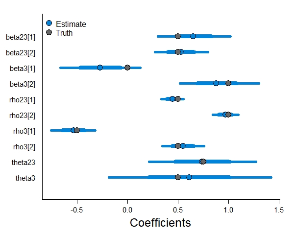
The model did a sufficient job retrieving the parameter estimates, the horizontal lines are 95% credible intervals and the true values fall within them. Note that we are less certain in our estimates for the two autologistic terms, and that the autologistic term that only applies to state 3 (theta3) has the widest credible intervals. As the autologistic parameters depend on a state occurring in the previous time step, there is less data available to them in the model. As a result, there is more parameter uncertainty associated to them.
The next thing that I like to plot out is the expected occupancy from the TPM. I like doing this before plotting out the TPM as it helps you see the overall pattern, which helps me interpret the TPM results.
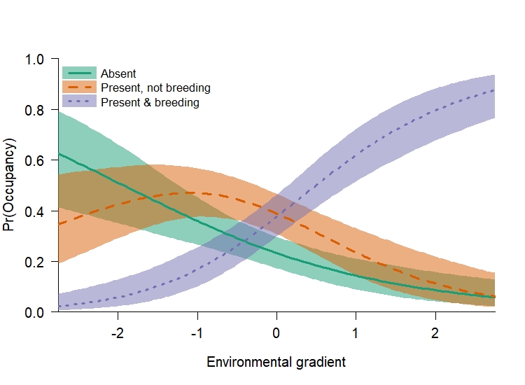
From this figure we can see that there is a portion of the landscape that each state is the most likely to occur. If we were going to write up the results from this model, how can we interpret our regression coefcients relative to this pattern? Understanding state 1 is simple, as it is \((1 - \omega)\). Because \(\omega\) had a positive slope term (0.5) that means species absence \((1 - \omega)\) should increase when the environmental gradient is negative. Interpretting the expected occupancy for states 2 and 3 is a little more difficult, because those states are associated to both \(\omega\) and \(\delta\). From our simulation, the slope term associated to \(\delta\) was 1.0, which means it was positive and of greater magnitude than the slope term for \(\omega\) (0.5). As such, both \(\omega\) and \(\delta\) should increase as the environmental covariate becomes more positive. Likewsie, \((1 - \delta)\) should increase when as the environmental covariate is negative. Because state 2 is \(\omega \times (1 - \delta)\), we are multiplying two probabilities that are highest at the opposite ends of the environmental gradient. Therefore, state 2 should be highest somewhere in the middle of the gradient. And Because state 3 is \(\omega \times \delta\), we are multiplying two probabilities that are highest at the positive end of the environmental gradient, which means it should be highest there.
Finally, we can plot out the TPM along our environmental gradient. Note that I’ve transposed the TPM so that columns are the “from this state” and the rows are the “to this state” of this 3x3 figure. One thing that is important to note about this class of model is that the autologistic terms do not change the direction of an effect, they only modify the intercept value of a given element of the TPM if they are present. Because I used relatively small theta values to simulate these data, we do not see much variation among the three states (i.e., comparing rows of the plot below).
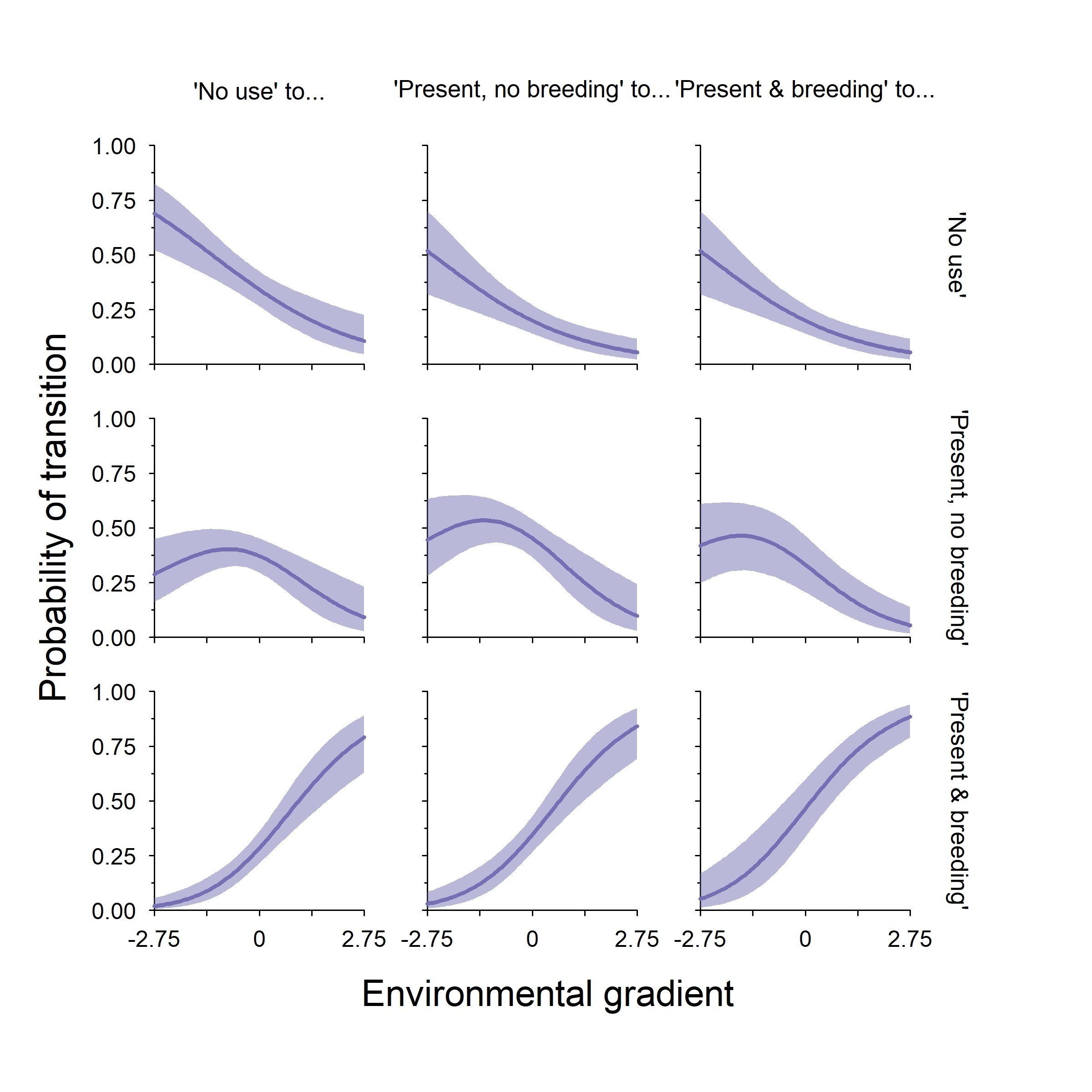
In this example (and with this class of model), the TPM tells a very similar story to the expected occupancy plot. As such, I probably would not include the latter in a manuscript. However, that is not always the case (as you will see in a later blog post for dynamic multistate models).
And that is how you fit this style of autologistic multistate occupancy model. It is the simplest version, as it only requires two additional parameters to fit a dynamic model. Let’s move on to the softmax model now and add a little more complexity. Check out all the code to simulate, fit, and plot the results here.
An autologistic multistate model occupancy that uses the softmax function
I’m assuming you have read my first post on multistate models and therefore are familiar with the softmax function. If you have not, you can read it here. I am going to add a little more complexity to the model and use four autologistic parameters instead of two. As such, the latent state TPM of this model is:
\[\boldsymbol{\psi_{s,t}} = \begin{bmatrix} \psi_{s,t}^1 & \psi_{s,t}^{2} & \psi_{s,t}^3 \\ \psi_{s,t}^{1|2} & \psi_{s,t}^{2|2} & \psi_{s,t}^{3|2} \\ \psi_{s,t}^{1|3} & \psi_{s,t}^{2|3} & \psi_{s,t}^{3|3} \end{bmatrix}\]Where each row sums to one. The seperate probabilities in our TPM can be defined as:
- \(\psi_{s,t}^1\): The probability the species is absent at site s at time t given the species was not present at t-1 (or if t=1).
- \(\psi_{s,t}^2\): The probability the species is present but not breeding at site s at time t given the species was not present at t-1 (or if t=1).
- \(\psi_{s,t}^3\): The probability the species is present and breeding at site s at time t given the species was not present at t-1 (or if t=1).
- \(\psi_{s,t}^{1|2}\): The probability the species is absent at site s at time t given the state was 2 at t-1.
- \(\psi_{s,t}^{2|2}\): The probability the species is present but not breeding at site s at time t given the state was 2 at t-1.
- \(\psi_{s,t}^{3|2}\): The probability the species is present and breeding at site s at time t given the state was 2 at t-1.
- \(\psi_{s,t}^{1|3}\): The probability the species is absent at site s at time t given the state was 3 at t-1.
- \(\psi_{s,t}^{2|3}\): The probability the species is present but not breeding at site s at time t given the state was 3 at t-1.
- \(\psi_{s,t}^{3|3}\): The probability the species is present and breeding at site s at time t given the state was 3 at t-1.
Just like the previous model we assume that the latent state z is a categorical random variable. At t=1 we use the first row of the TPM because we have no prior knowledge on the state of a site before sampling
\[z_{s,t=1} \sim \text{Categorical}(\boldsymbol{\psi_{s,1}})\]and we condition the rest of the years of sampling on the state of a site at t-1
\[z_{s,t} \sim \text{Categorical}(\boldsymbol{\psi_{s,z_{s,t-1}}}), t>1\]The detection matrix for the data model is:
\[\boldsymbol{\eta}_{s,j} = \begin{bmatrix} 1 & 0 & 0 \\ (1 - \rho_{s,j}^{2|2}) & \rho_{s,j}^{2|2} & 0 \\ \rho_{s,j}^{1|3} & \rho_{s,j}^{2|3} & \rho_{s,j}^{3|3} \end{bmatrix}\]where \(\rho_{s,j}^{1|3} = 1 - \rho_{s,j}^{2|3} - \rho_{s,j}^{3|3}\). Here we assume that detecting state 2 when the true state is 3 (\(\rho_{s,j}^{2|3}\)) is not the same as detecting state 2 when the true state is 2 (\(\rho_{s,j}^{2|2}\)). This could be because the behavior of our species is different when it is and is not breeding such that their detection probability differs. Using this matrix, the data model is
\[y_{s,j,t} \sim \text{Categorical}(\boldsymbol{\eta}_{s,j,z[s]})\]where the latent state z at time t indexes the appropriate row of the detection probability matrix.
We are going to use the softmax function to add linear predictors to this model. Therefore, we need to specify one probability in each row of our matrices to be a reference category. For the latent state TPM the natural choice is state 1 (species absence). One way I like to write out the linear predictors for a TPM that uses softmax is to create a new matrix that stores the numerator of the softmax function for each transition. That way all we need to do is divide each row by it’s sum to finish the softmax function. For this model, let \(\boldsymbol{\phi_{s,t}}\) be an array with the same dimensions as \(\boldsymbol{\psi_{s,t}}\). Remembering that exp(0) = 1, our linear predictor matrix is:
\[\boldsymbol{\phi_{s,t}} = \begin{bmatrix} 1 & \text{exp}(\boldsymbol{\beta}^2 \boldsymbol{x}_s) & \text{exp}(\boldsymbol{\beta}^3 \boldsymbol{u}_s) \\ 1 & \text{exp}(\boldsymbol{\beta}^{2|2} \boldsymbol{x}_s + \theta^{2|2}) & \text{exp}(\boldsymbol{\beta}^{3|2} \boldsymbol{u}_s + \theta^{3|2}) \\ 1 & \text{exp}(\boldsymbol{\beta}^{2|3} \boldsymbol{x}_s + \theta^{2|3}) & \text{exp}(\boldsymbol{\beta}^{3|3} \boldsymbol{u}_s + \theta^{3|3}) \end{bmatrix}\]Where we have four autologistic terms in the bottom two rows, and one design matrix for states 2 and 3 (respectively X and U, both of which have a vector of 1’s in the first column to account for the model intercept). To create our TPM from this matrix of linear predictors all we need to do is divide each element in a given row by the summation of that row.
Using the same approach, the linear predictors for the detection matrix are:
\[\boldsymbol{\eta}_{s,j} = \begin{bmatrix} 1 & 0 & 0 \\ 1 & \text{exp}(\boldsymbol{\alpha}^{2|2} \boldsymbol{k}_{s,j}) & 0 \\ 1 & \text{exp}(\boldsymbol{\alpha}^{2|3} \boldsymbol{k}_{s,j}) & \text{exp}(\boldsymbol{\alpha}^{3|3} \boldsymbol{k}_{s,j}) \end{bmatrix}\]Where \(\boldsymbol{\alpha}\) is a vector of parameters and k is the detection design matrix. Remember that we cannot detect state 3 when the true state is 2, so we place a zero in that part of the matrix. To create our detection probability matrix from this detection linear predictor matrix all we need to do is divide each element in a given row by the summation of that row.
Finally, for the parameter model (the priors) we can give every parameter vague Logistic(0,1) priors.
The softmax model written in JAGS
The softmax model with four autologistic priors can be written like this in JAGS, which is the file ./JAGS/autologistic_multistate_softmax.R on this repository.
model{
  #
  #THE LATENT STATE MODEL
  #
  for(site in 1:nsite){
    # LATENT STATE LINEAR PREDICTORS.
    #   Note: I am assuming here that while the model is dynamic,
    #   The probabilities do not vary by year (because the
    #   linear predictors do not vary through time).
    #
    # latent state probabilities given state == 1 (or t = 1)
    psi[site,1,1] <- 1
    psi[site,1,2] <- exp( inprod(beta2, x[site,] ) )
    psi[site,1,3] <- exp( inprod(beta3, u[site,] ) )
    # latent state probabilities given state == 2
    psi[site,2,1] <- 1
    psi[site,2,2] <- exp( inprod(beta2, x[site,] ) + theta2g2 )
    psi[site,2,3] <- exp( inprod(beta3, u[site,] ) + theta3g2 )
    # latent state probabilities given state == 3
    psi[site,3,1] <- 1
    psi[site,3,2] <- exp( inprod(beta2, x[site,] ) + theta2g3 )
    psi[site,3,3] <- exp( inprod(beta3, u[site,] ) + theta3g3 )
    # Estimate latent state year == 1. Setting to first
    #  row of psi because we have no prior knowledge
    #  on state of site before we started sampling.
    z[site,1] ~ dcat(
      psi[site,1,] / sum(psi[site,1,])
    )
    # Do the remaining years. We grab the correct row
    #  of the transition matrix based on the state in the
    #  previous time step.
    for(year in 2:nyear){
      z[site,year] ~ dcat(
        psi[site,z[site,year-1],] / sum(psi[site,z[site,year-1],])
      )
    }
  }
  #
  # THE DATA MODEL
  #
  for(site in 1:nsite){
    for(survey in 1:nsurvey){
      # Set up the logit linear predictors
      #   Note: I am assuming here that while the model is dynamic,
      #   The probabilities do not vary by year (because the
      #   linear predictors do not vary through time).
      # Fill in detection probability matrix
      # First row: TS = 1
      eta[site,survey,1,1] <- 1 # -------------------------------------- OS = 1
      eta[site,survey,1,2] <- 0 # -------------------------------------- OS = 2
      eta[site,survey,1,3] <- 0 # -------------------------------------- OS = 3
      # Second row: TS = 2
      eta[site,survey,2,1] <- 1 # -------------------------------------- OS = 1
      eta[site,survey,2,2] <- exp( inprod( rho2g2, k[site,survey,] ) ) # OS = 2
      eta[site,survey,2,3] <- 0 # -------------------------------------- OS = 3
      # Third row: TS = 3
      eta[site,survey,3,1] <- 1 # -------------------------------------- OS = 1
      eta[site,survey,3,2] <- exp( inprod( rho2g3, k[site,survey,] ) ) # OS = 2
      eta[site,survey,3,3] <- exp( inprod( rho3g3, k[site,survey,] ) ) # OS = 3
      for(yr in 1:nyear){
        # Index the appropriate row of eta based on the current latent state.
        # Again, we are assuming there is no variation among years or sampling.
        y[site,survey,yr] ~ dcat(
          eta[site,survey,z[site,yr],] / sum(eta[site,survey,z[site,yr],])
        )
      }
    }
  }
  #
  # Priors
  #
  # Pr(latent state 2)
  for(b2 in 1:nbeta2){
    beta2[b2] ~ dlogis(0,1)
  }
  # Pr(latent state 3)
  for(b3 in 1:nbeta3){
    beta3[b3] ~ dlogis(0,1)
  }
  # Autologistic terms
  theta2g2 ~ dlogis(0,1)
  theta3g2 ~ dlogis(0,1)
  theta2g3 ~ dlogis(0,1)
  theta3g3 ~ dlogis(0,1)
  # Pr(OS = 2 | TS = 2)
  for(ts2 in 1:nts2){
    rho2g2[ts2] ~ dlogis(0,1)
  }
  # Pr(OS = 2 | TS = 3) & Pr(OS = 3 | TS = 3)
  for(ts3 in 1:nts3){
    rho2g3[ts3] ~ dlogis(0,1)
    rho3g3[ts3] ~ dlogis(0,1)
  }
}
Simulating some data and plotting the results from the softmax model
Because we specified four autologistic terms, I had to increase the sample size of this simulation (more sites and more years) to accurately estimate them. The reason for this is because we need a sufficient sample size of each transition (e.g., state 2 to state 3) in order to estimate them, which can be difficult. For reference, there are two steps you could take if you wanted to simplify this model and make it more like the logit-link model parameterization (i.e., 2 autologistic parameters instead of 4). First, for row 2 of the TPM we would create a new \(\theta^2\) parameter and replace both autologistic parameters in that row with it. Second, for row 3 we would create a new \(\theta^3\) parameter and replace both autologistic parameters in that row with it.
The script to simulate and fit an autologistic multistate softmax model is ./R/examples/autologistic_softmax_example.R in this repository. This script also includes the code to make the three figures in this section, so look there if you are interested in seeing how I made them.
# The autologistic multistate occupancy model using softmax

library(runjags)
library(mcmcplots)
library(markovchain)

# Note: I parameterized this model complex than the aulogistic model
#       that used the logit link. I only did this to show how
#       there are different assumptions you can make with this model.
#       This does, however, make this model much more data hungry.
#       And it's not so much overall sample size, it's the number of
#       transitions among different states!

# Load all the functions we need to simulate the data
sapply(
  list.files("./R/functions", full.names = TRUE),
  source, verbose = FALSE
)

# -------------------------------------------
# Autologistic model that uses softmax
# -------------------------------------------

# General bookkeeping
nsite <- 100
nsurvey <- 8
nyear <- 6
set.seed(188)

# OS = observed state
# TS = true state

my_params <- list(
  # latent state 2 parameters
  beta2 = c(-0.5,0.5),
  # latent state 3 parameters
  beta3 = c(-1,2),
  # detection, OS=2|TS=2
  rho2g2 = c(0.5,1),
  # detection, OS=2|TS=3
  rho2g3 = c(0.75,0),
  # detection, OS=3|TS=3
  rho3g3 = c(1,-0.5),
  # autologistic, 2 given 2 at t-1
  theta2g2 = 0.75,
  # autologistic, 3 given 2 at t-1
  theta3g2 = 2,
  # autologistic, 2 given 3 at t-1
  theta2g3 = -0.5,
  # autologistic, 3 given 3 at t-1
  theta3g3 = 0.5,
  nyear = nyear
)

# For latent state being either 2 or 3
x <- cbind(1, rnorm(nsite))
# For conditional probability site is in state 3
u <- x

# for detection data model. Assuming the same
#  design matrix for all parameters.
k <- array(1, dim = c(nsite, nsurvey,2))

# Some sort of covariate that varies across
#  surveys. Note that if you also have covariates
#  that do not vary across surveys you just repeat
#  the values across the second dimension of k.
k[,,2] <- rnorm(nsite * nsurvey)

# Make a list for covariates
my_covs <- list(
  beta2 = x,
  beta3 = u,
  rho2g2 = k,
  rho2g3 = k,
  rho3g3 = k
)

# simulate data
y <- simulate_autologistic(
  params = my_params,
  covs = my_covs,
  link = "softmax"
)

transitions(y)

# make the data list for modeling
data_list <- list(
  # observed data
  y = y,
  # design matrices
  x = x,
  u = u,
  k = k,
  # for looping
  nsite = nsite,
  nsurvey = nsurvey,
  nyear = nyear,
  # number of parameters for different
  #  linear predictors
  nbeta2 = length(my_params$beta2),
  nbeta3 = length(my_params$beta3),
  nts2 = length(my_params$rho2g2),
  nts3 = length(my_params$rho3g3)
)

# fit the model
m1 <- run.jags(
  model = "./JAGS/autologistic_multistate_softmax.R",
  monitor = c("beta2", "beta3", "rho2g2", "rho2g3",
              "rho3g3", "theta2g2", "theta3g2",
              "theta2g3", "theta3g3"),
  data = data_list,
  n.chains = 4,
  inits = init_autologistic_softmax,
  adapt = 1000,
  burnin = 20000,
  sample = 10000,
  modules = "glm",
  method = "parallel"
)

# summarise model
msum <- summary(m1)

# save output for later
saveRDS(m1, "autologistic_softmax_mcmc.rds")
Just like with the logit-link model, our softmax parameterization with four autologistic terms did a good job estimating the true parameters (though I added an extra two years of sampling and 25 sites to do so).
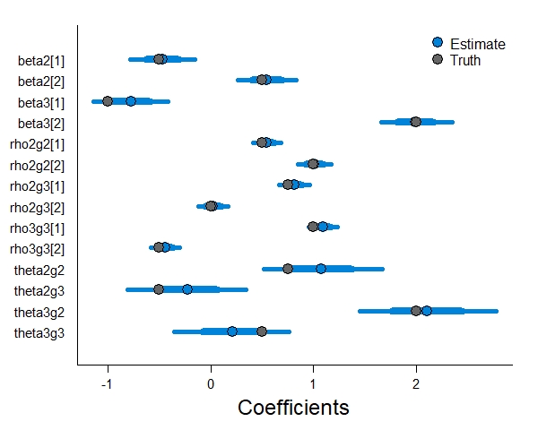
Just like the last model, let’s plot out the expected occupancy of each state first. We have much more data here, so our credible intervals have gotten much smaller.
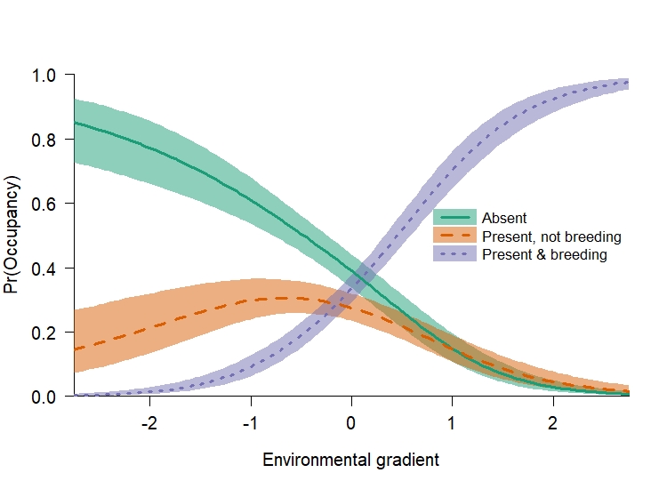
Unlike the previous simulation, the two most likely states along our gradient are either “species absence” or “present and breeding”. However, there is still a portion of the landscape (at negative values of our gradient), where this species occurs with a relatively low probability and does not breed.
How are the parameters we used to simulate these data causing this pattern? It’s mostly the difference in magnitude between the two positive slope terms for state 2 (0.5) and state 3 (2). As a reminder, the softmax function divides each linear predictor in a row of the TPM by the row sum. Ignoring intercept values and autologistic terms, 2 / (0.5 + 2) > 0.5 / (0.5 + 2). Therefore, when the environmental gradient is positive state 3 is most likely. Likewise, when the environmental gradient is negative state 2 becomes more likely than state 3. However, state 1 is most likely to occur when the environmental gradient is negative because the slope terms for state 2 and 3 are positive.
Finally, we can plot out the TPM along our environmental gradient. Note that I’ve transposed the TPM so that columns are the “from this state” and the rows are the “to this state” of this 3x3 figure. One thing that is important to note about this class of model is that the autologistic terms do not change the direction of an effect, they only modify the intercept value of a given element of the TPM if they are present.
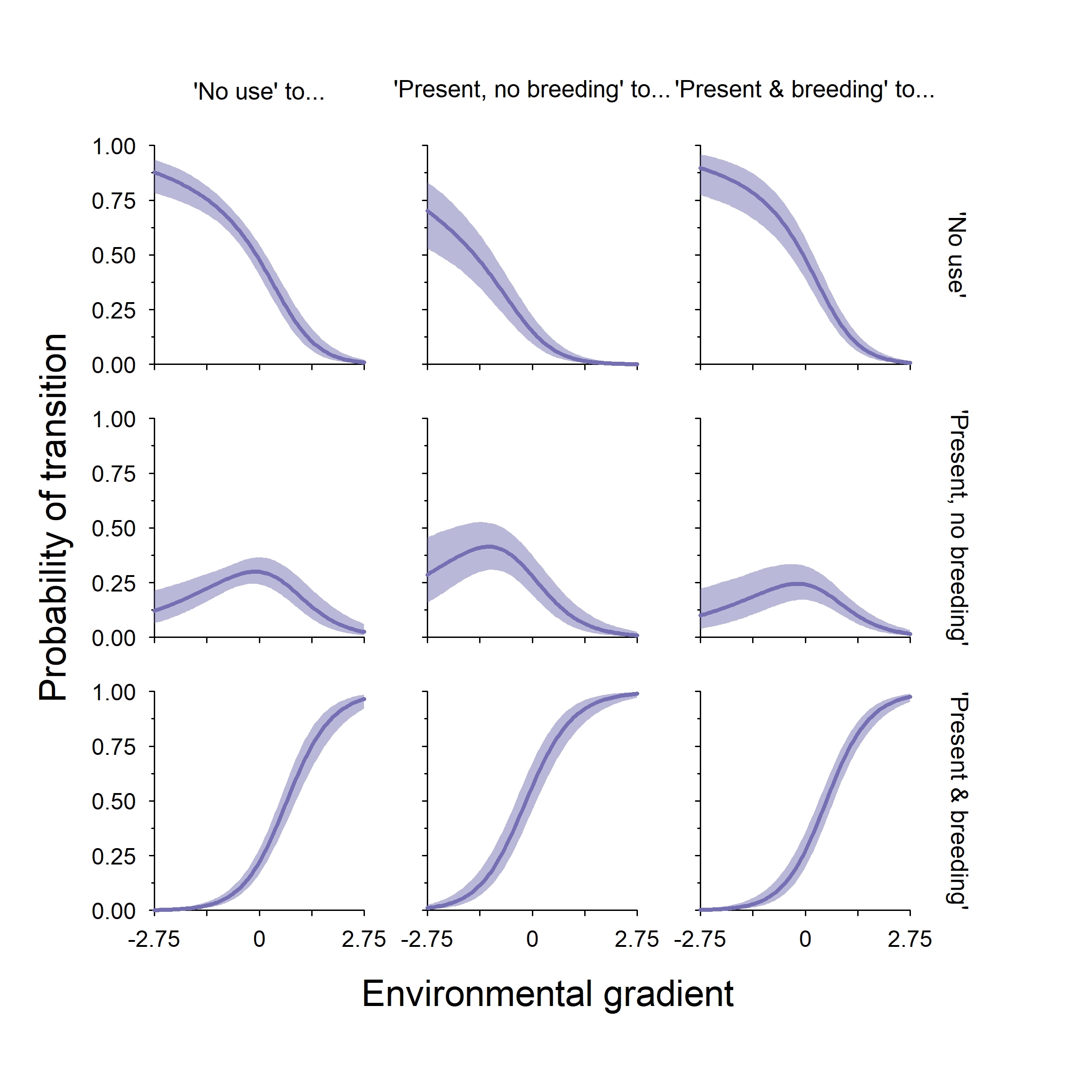
We see a little more variation in this model across rows than we did with the logit-link model, but that is only because I used larger autologistic terms. However, there is not that much variation. And that is how you fit two different styles of autologistic multistate occupancy models!
All code for this multistate modeling series is located here.