Mason Fidino

Dynamic occupancy models can estimate local colonization (\(\gamma\)) and extinction (\(\epsilon\)) rates and are incredibly powerful, but data hungry tools. For example, simulation studies have suggested that a minimum of 120 unique sampling locations are necessary to accurately estimate both \(\gamma\) and \(\epsilon\)! In my experience, most occupancy studies sample far fewer than 120 sites over time, and so there is generally some uncertainty in how to model these data. Generally speaking, it would not be a good idea to fit a static occupancy model to all of the data for a couple reasons. First, doing so is pseudoreplication, and the resulting standard errors for your parameter estimates will be too precise. Second, fitting a standard single season occupancy model to multiple years of data fails to account for any potential temporal dependence among years. For example, if Virginia opossum (Didelphis virginiana) were present at one survey location in year 1, there may be a higher probability they are present in year 2. So, what do you do?

Instead of fitting a dynamic occupancy model, one common suggestion is to use a ‘stacked design’ and fit a static occupancy model with a random site effect. This can be a very appropriate technique, however it may have some of the same issues as fitting a dynamic occupancy model, namely the introduction of a potentially large number of parameters to be estimated (one for each site sampled). An arguably simpler model is the auto-logistic formulation of an occupancy model, which includes a first-order autoregressive term to account for temporal dependence between primary sampling periods. This model has seen some attention in the literature (1, 2, 3), but not as much as I think it should. As such, I’ll walk through what this model is, provide a simulated example, and fit the model in JAGS.

The auto-logistic occupancy model

Let \(\Psi\) be the probability of occupancy and z be a Bernoulli random variable that equals 1 if a the species is present and 0 if it is absent. For i in 1,…,I sites and t in 1,…,T years, the probability of occupancy when t = 1 is:

where \(\pmb{\beta}\pmb{x}_i\) represents a vector of regression coefficients (including the model intercept) and their associated covariates. This part of the model should look incredibly standard, because it is the latent state of a static occupancy model. For t>1 however, we need to account for temporal dependence between years. To do so, we introduce \(\theta\) into the model, which is a first-order autoregressive term. Thus, for the remaining years of sampling, the logit-linear predictor is then:

Thus, the \(\theta\) term in this model here helps us determine if species presence in the previous timestep is associated to species presence in the current time step. And while the auto-logistic model does have this new \(\theta\) term in the latent state model, there is not much that changes with the data model. Let \(\rho\) be the conditional probability of detection, \(y_{i,t}\) be the number of secondary sampling occasions (hereafter days) the species was detected at site i and year t, and \(J_{i,t}\) be the total number of days sampled at site i and year t . This level of the model is then:

Like the latent state linear predictor, this level of the model also includes regression coefficients and their associated covariates (\(\pmb{\alpha}\pmb{x}_i\)), which may or may not be the same as what are included in the latent state model. What is nice about this model is that it only includes one new parameter, \(\theta\), and it does not have any random effects which makes it simpler to interpret. From this model, the average occupancy probability is a little different than a standard static occupancy model. Assuming covariates are mean-centered, it can be derived as:

where expit is the inverse logit function and \(\beta_0\) is the occupancy intercept. Likewise, site-specific predictions can also be derived by including the respective slope terms and covariates into the above equation.

A simulated example

For this simulation we are going to assume we have monitored 25 sites for 8 primary sampling periods (e.g., years, seasons, etc.). This, of course, is way below the recommendation for fitting a dynamic occupancy model, so let’s see how the auto-logistic model performs (we could make this model fit really well if we did more sites, but that is not the motivation here). Let’s also assume we are trying to fit three covariates on \(\Psi\) and \(\rho\), which is about the maximum I would be comfortable with given this amount of data.

# Step 1. Simulate the data.

# General bookkeeping
nsite <- 25
nyear <- 8
ncovar <- 3
nrepeats <- 5

# for covariates
X <- matrix(
  NA,
  ncol = ncovar,
  nrow = nsite
)

set.seed(333)
# Create covariates
X <- cbind(1,apply(X, 2, function(x) rnorm(nsite)))

# Occupancy coefficients, +1 for intercept
psi_betas <- rnorm(ncovar + 1)

# auto-logistic term
theta <- 0.75

# Detection coefficients, decreasing magnitude here
rho_betas <- rnorm(ncovar + 1, 0, 0.5)

# latent state, give same dimensions as X
z <- matrix(NA, ncol = nyear, nrow = nsite)

# Do first year occupancy
psi <- plogis(X %*% psi_betas)
z[,1] <- rbinom(nsite, 1, psi)

# And then the rest, which also uses the theta term
for(year in 2:nyear){
  psi <- plogis(X %*% psi_betas + theta * z[,year-1])
  z[,year] <- rbinom(nsite,1,psi)
}

# Add imperfect detection, make it a matrix with
#  the same dimensions as z. Then multiply by z.
rho <- matrix(
  plogis(X %*% rho_betas),
  ncol = nyear,
  nrow = nsite
) * z

# Create the observed data. Again, same dimensions as z.
y <- matrix(
  rbinom(
    length(rho),
    nrepeats,
    rho
  ),
  ncol = nyear,
  nrow = nsite
)

And now we have our simulated data y and covariates X that we can use to fit out model. In JAGS, the auto-logistic model can be written as:

model{
  for(site in 1:nsite){
    # This is for the first year
    #
    # latent state model
    #
    logit(psi[site,1]) <- inprod(psi_beta, X[site,])
    z[site,1] ~ dbern(psi[site,1])
    #
    # data model
    #
    logit(rho[site,1]) <- inprod(rho_beta, X[site,])
    y[site,1] ~ dbin(rho[site,1] * z[site,1], J)
    #
    # For remaining years of sampling
    #
    for(year in 2:nyear){
      #
      # latent state model, has theta term now.
      #
      logit(psi[site,year]) <- inprod(psi_beta, X[site,]) +
        theta * z[site,year-1]
      z[site,year] ~ dbern(psi[site,year])
      #
      # data model
      #
      logit(rho[site,year]) <- inprod(rho_beta, X[site,])
      y[site,year] ~ dbin(rho[site,year] * z[site,year], J)
    }
  }
  #
  # Priors
  #
  # Intercept and slope terms
  for(covar in 1:ncovar){
    psi_beta[covar] ~ dlogis(0,1)
    rho_beta[covar] ~ dlogis(0,1)
  }
  # First-order autoregressive term
  theta ~ dlogis(0,1)
}

which, on the GitHub repository for this post can be found at ./jags/autologistic_model.R.

Fitting the model

Now, we can fit the model in JAGS via the runjags package.

# data list for model
data_list <- list(
  J = nrepeats,
  nsite = nsite,
  nyear = nyear,
  X = X,
  ncovar = ncovar + 1, # for intercept
  y = y
)

# initial values
my_inits <- function(chain){
  gen_list <- function(chain = chain){
    list(
      z = matrix(1, ncol = data_list$nyear, nrow = data_list$nsite),
      psi_beta = rnorm(data_list$ncovar),
      rho_beta = rnorm(data_list$ncovar),
      theta = rnorm(1),
      .RNG.name = switch(chain,
                         "1" = "base::Wichmann-Hill",
                         "2" = "base::Wichmann-Hill",
                         "3" = "base::Super-Duper",
                         "4" = "base::Mersenne-Twister",
                         "5" = "base::Wichmann-Hill",
                         "6" = "base::Marsaglia-Multicarry",
                         "7" = "base::Super-Duper",
                         "8" = "base::Mersenne-Twister"),
      .RNG.seed = sample(1:1e+06, 1)
    )
  }
  return(switch(chain,
                "1" = gen_list(chain),
                "2" = gen_list(chain),
                "3" = gen_list(chain),
                "4" = gen_list(chain),
                "5" = gen_list(chain),
                "6" = gen_list(chain),
                "7" = gen_list(chain),
                "8" = gen_list(chain)
  )
  )
}

# fit the model
my_mod <- runjags::run.jags(
  model = "./jags/autologistic_model.R",
  monitor = c("theta", "psi_beta", "rho_beta"),
  data = data_list,
  inits = my_inits,
  n.chains = 4,
  adapt = 1000,
  burnin = 10000,
  sample = 10000,
  method = "parallel"
)

# model summary
my_sum <- summary(my_mod)

Overall, the model converges nicely, and does an okay job returning the model coefficients. Certainly, with additional data (i.e., sites sampled per year) we would expect the precision of the estimates to improve. Plotting out the estimated values (blue dots & lines) with the simulated values (yellow dots) shows that they all fall within each parameters 95% credible interval.

caterplot(
  my_mod,
  collapse = TRUE,
  reorder = FALSE
)

points(
  x =  c(theta, psi_betas, rho_betas),
  y = rev(1:9),
  pch = 21,
  bg = "yellow",
  cex = 1.2
)

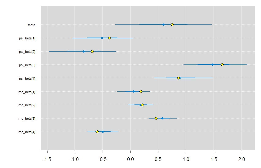
And there you have it. An occupancy model that can account for temporal dependence between sampling periods with a single parameter! Definitely something to have in your modelers toolkit for when you may not have enough data for a dynamic occupancy model.

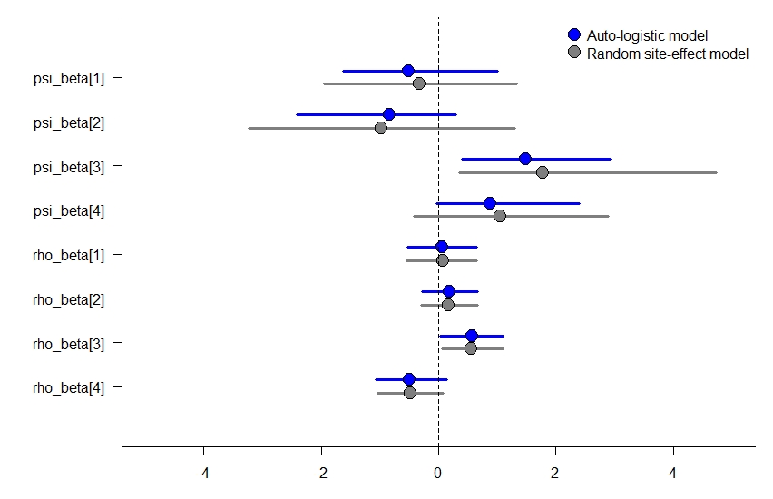
How does this compare to a stacked model with a random effect?

While I’m not going to walk through the formulation of the stacked design occupancy model with a site-level random effect, I did go ahead and fit it to the simulated data above to see how much the parameter estimates changed for the occupancy slope terms. Overall, they look about the same, though the site-level random effect model has slightly wider credible intervals, which may be a better reflection of these data. You can see the code for fitting the stacked model here.