An introduction to multistate occupancy models. A static three-state model for one species.

I’ve got a little bone to pick with the term multistate occupancy model.

As the name implies, multistate occupancy models estimate multiple states across space and sometimes through time (e.g., species absent, species present but not breeding, species present and breeding). However, every occupancy model estimates multiple states. A static single-season occupancy model, for example, estimates species presence with \(Pr(\psi)\) and absence with \(1 - Pr(\psi)\). As long as \(Pr(\psi)\) is not 0 or 1, there will be locations where we expect the species to be or not to be, and therefore there are multiple states.

Should we rename these models? Absolutely not, but we could be more specific about what makes this class of model unique. Multistate models have earned their name because they partition the probability of success (e.g., species presence) into multiple discrete states. Standard occupancy models do not do that. Two common examples for single-species multistate models include splitting species presence into breeding & non-breeding states (Nichols et al. 2007) or healthy & not healthy states (Murray et al. 2021). For multi-species models, you can even estimate separate community states (e.g., species A only, species B only, species A&B together; Fidino et al. 2018). Because of their wide ranging applications, multistate models are an incredibly versatile tool you can use to answer a variety of ecological questions. However, this versatility can make it confusing to learn how multistate models work and how to interpret their results, especially because the models can be written up in multiple ways (statistically speaking).

Regardless of how a multistate model is written, I would say that they can be described by three key features, which I will call the central tenants of multistate occupancy models:

There are at least three states being modeled, one of which is always “species absence.” The interpretation of the remaining states depends on the model & data, but these states are always related to species presence in one form or another.
There is a separate probability of ‘success’ for each state, including species absence.
The sum of the probabilities across all states must sum to unity (i.e., sum to 1).

In this first of what will be multiple posts about multistate models, I am going to introduce the simplest multistate model there is: a static three-state occupancy model for a single species. I will also show how to include covariates in this model with the softmax function (link to wikipedia). The softmax function is a generalization of the inverse logit link that can accommodate any number of categories (i.e., states), and can convert multiple linear predictors into a set of probabilities that fulfill the central tenants of multistate models. For all of the simulation code & JAGS implementations of these models, visit this GitHub repository here.

Links to the different sections of this post

The static multistate occupancy model
Including covariates with the softmax function
Fitting the multistate occupancy model in JAGS
Plotting out the results from your model

Before I get started with the model formulation, lets add some ecological motivation to this example. So, let’s assume we have decided to study great horned owl (Bubo virginianus) and want to estimate their distribution and reproductive rate throughout Chicago, Illinois, USA.

The static multistate occupancy model

For our owl study assume we have conducted j in 1,…,J surveys at s in 1,…,S sites throughout Chicago, Illinois during the breeding season for great horned owls. During each of these surveys we can record 1 of 3 possible values:

No detection of an owl
Detection of an adult owl but no detection of a young owl
Detection of a young owl (i.e., reproductive success)

We store these observations in the S by J matrix \(\boldsymbol{Y}\) (this is in upper case and bold because it is a matrix). What this means is that we are interested in quantifying three separate states: owls are not present (state = 1), owls are present but not breeding (state = 2), and owls are present and breeding (state = 3). Note that if the true state at a site is 1 (owls not present), then we could never observe owls there. Likewise, if the true state is 2 (owls present but not breeding), then it’s possible for us to observe either state 1 because we failed to detect the owl or state 2 because we did. Finally, we have the opportunity to observe all three states if the true state at a site is 3 (owls present and breeding).

To estimate the true state at a site we must specify a probability for each state. There are a couple of ways to do this. One way would be:

\[\boldsymbol{\psi_s} = \begin{bmatrix}(1-\omega_s) & \omega_s(1-\delta_s) & \omega_s\delta_s\end{bmatrix}\]

where \(\omega_s\) is the probability owls occupy site s regardless of breeding status and \(\delta_s\) is the conditional probability that owls are breeding at site s given they are present. This representation fufills the central tenants of multistate models, and one nice feature of this representation is that \(\omega_s\) and \(\delta_s\) can take value between 0 and 1 \(\boldsymbol{\psi_s}\).

# create a sequence of values from 0 to 1
#  for omega and delta
omega <- seq(0,1,0.01)
delta <- seq(0,1,0.01)

# Get every possible combination
#  of values for omega and delta.
all_combos <- expand.grid(
  omega,
  delta
)

# go through all the combinations
#  using the equation from above.
psi <- apply(
  all_combos,
  1,
  function(x) c(
    1-x[1],
    x[1] * (1 - x[2]),
    x[1] * x[2]
  )
)

# Look at first few values,
#  which all sum to 1.
head(colSums(psi))
[1] 1 1 1 1 1 1

# In fact,all values equal 1!
table(colSums(psi)) == nrow(all_combos)
    1 
10201 

The other way I have seen the latent states probabilities written out is:

\[\boldsymbol{\psi_s} = \begin{bmatrix} \psi_s^1 & \psi_s^2 & \psi_s^3\end{bmatrix}\]

where \(\psi_s^1\) is the probability owls do not occupy site s, \(\psi_s^2\) is the probability owls are present but not breeding, and \(\psi_s^3\) is the probability owls are present and breeding. To make this vector fulfill the central tenants of multistate models, let \(\psi_s^1 = 1 - \psi_s^2 - \psi_s^3\) . However, unlike the first representation \(\psi_s^2\) and \(\psi_s^3\) cannot be any number between 0 and 1 as there are combinations that would make sure that the \(\Sigma_{m=1}^3 \boldsymbol{\psi_s^m} \neq 1\). This is okay, as you will later see we can ensure that whatever gets estimated sums to 1 within the model. In this case, I’m going to use the second representation for this model presentation because it is a little more general and therefore easier to abstract out to more than three states (if that was something you wanted to do). Another difference with this representation is that the marginal occupancy of owls (i.e., their distribution) is \(\psi_s^2 + \psi_s^3\) (i.e., the probability a site has owls that are not breeding plus the probability a site has breeding owls).

Let \(z_s\) be the latent state of site s, which can either equal 1, 2, or 3. For Bayesian multistate models, we assume that \(z_s\) is a Categorical random variable. The Categorical distribution, which is a generalization of the Bernoulli distribution, is a discrete probability distribution that describes the potential results of a random variable that can take of one of m categories, which is exactly what we need. Therefore, we can write the latent state model as

\[z_s \sim \text{Categorical}(\boldsymbol{\psi_s})\]

However, we observe \(z_s\) with error, and so need to account for that in the data model. As a reminder, state uncertainty changes depending on what state was observed, which is possibly the most confusing part of this model. In my opinion, the easiest way to represent the varying detection probabilities is to put them into a matrix where each row denotes the true state of \(z_s\) and each column denotes the probability of detecting each state given the true state. For this owl model, the detection matrix is:

\[\boldsymbol{\eta_s} = \begin{bmatrix} 1 & 0 & 0 \\ (1 - \rho_s^{2,2}) & \rho_s^{2,2} & 0 \\ \rho_s^{1,3} & \rho_s^{2,3} & \rho_s^{3,3} \end{bmatrix}\]

For our three state model we end up with the 3 x 3 matrix \(\boldsymbol{\eta_s}\) where each row of meets the central tenants of multistate models. To walk through this, if we are in state 1 (owls not present, the first row of \(\boldsymbol{\eta_s}\)), it is impossible to observe state 2 or 3 because owls are literally not there. Therefore, the probability we observe state “owls not present” given the true state is “owls not present” must be 1. When the true state is state 2 (owls present but not breeding, the second row of \(\boldsymbol{\eta_s}\)), then we could possibly observe either state 1 or 2. As such, we detect state 1 with \(Pr(1 - \rho_s^{2,2})\) and state 2 with \(Pr(\rho_s^{2,2})\). If the true state is 2, then we cannot observe state 3. Finally, if the true state is state 3 (owls present and breeding) it is possible to observe all three states. Just like with \(\boldsymbol{\psi_s}\), let \(\rho_s^{1,3} = 1 - \rho_s{2,3} -\rho_s{3,3}\) (i.e., the probability we detect state 1 is 1 minus the probability of detecting either of the two other states). To finish this off we detect state 2 with \(Pr(\rho_s^{2,3})\) and state 3 with \(Pr(\rho_s^{3,3})\).

For the data model, we also make use of the Categorical distribution such that:

\[y_{s,j} \sim \text{Categorical}(\boldsymbol{\eta}_{s,z[s]})\]

where \(z[s]\) indexes the appropriate row of the detection array. For example, if \(z[s] = 2\), then we would index the second row of \(\boldsymbol{\eta_s}\).

For a static multistate model without covariates, the last thing we need to do is specify priors. To give vague priors to \(\boldsymbol{\psi}\) and the third row in \(\boldsymbol{\eta_s}\), we can use a Dirichlet(1,1,1) prior for each. The Dirichlet distribution is a generalization of the Beta distribution for up to m categories, and in this case m = 3. The only other parameter in the model is \(\rho^{2,2}\), which we can give a vague Beta(1,1) prior.

Including covariates

As I said at the beginning of this post the softmax function is a generalization of the inverse logit link, and we can use it to add covariates into our multistate model. The softmax function is:

\[\text{softmax}(x) = \frac{\text{exp}(x)}{\sum_{i=1}^m \text{exp}(x)}\]

Where x is a vector of length m that contains the linear predictors for the m states at site s. However, one very important aspect to know is that if you have m states you only specify m-1 linear predictors. We must set one state as a reference category, and to do so we give that element in x a value of 0. Is this rule something new? Absolutely not, we also do this whenever we use the logit link. In fact, if you look at the inverse logit link function you can see pretty quickly that the ‘failure’ reference category has been baked into it (it’s the 1 in the denominator, remembering that exp(0) = 1). Thus, the inverse logit link:

\[\text{logit}^{-1}(x) = \frac{\text{exp}(x)}{1 + \text{exp}(x)}\]

could also be written as

\[\text{logit}^{-1}(x) = \frac{\text{exp}(x)}{\text{exp}(0) + \text{exp}(x)}\]

With a little bit more algebraic manipulation, you can hopefully see that the inverse logit is just the softmax function for 2 states written in a way that we only need to input the one linear predictor instead of a vector of length m. We could also, however, still use softmax for logistic regression if we wanted to:

# The softmax function. Convert any number of linear
#  predictors to a probability!
#
# arguments
#
# x = The linear predictors. One of these must be the
#       the baseline category (which equals zero.)  
#
softmax <- function(x){
  if(sum(x == 0) == 0){
    stop("No reference category. One value in x must equal zero.")
  }
  exp(x) / sum(exp(x))
}

# logit probability for 
#  failure and success
#  of some trial.
logit_probs <- c(0, 1)

# convert to probability
#  with softmax
softmax(logit_probs)
[1] 0.2689414 0.7310586

# which sums to 1
sum(softmax(logit_probs))
[1] 1

# try it with > 2 states
logit_multistate <- c(0,1,-0.5)

softmax(logit_multistate)
[1] 0.2312239 0.6285317 0.1402444

sum(softmax(logit_multistate))
[1] 1

Thus, we can use softmax to generate linear predictors for two of our three states, and then the final state gets estimated as 1 minus the sum of the other two probabilities. Additionally, the softmax function ensures our separate probabilities sum to 1, which is exactly what we need to fulfill the central tenants of multistate occupancy models. In regards to a reference category in our model, the natural choice is the first state (owls absent). So, for example, we can make the \(\boldsymbol{\psi_s}\) be a function of covariates with softmax, using separate design matrices for the two linear predictors (\(\boldsymbol{X}\) for state 2, \(\boldsymbol{U}\) for state 3).

\[\begin{eqnarray} \psi_s^1 &=& \frac{\phi_s^1}{\phi_s^1 + \phi_s^2 + \phi_s^3} \nonumber\\ \psi_s^2 &=& \frac{\phi_s^2}{\phi_s^1 + \phi_s^2 + \phi_s^3} \nonumber\\ \psi_s^3 &=& \frac{\phi_s^3}{\phi_s^1 + \phi_s^2 + \phi_s^3} \nonumber \end{eqnarray}\]

where

\[\begin{eqnarray} \phi_s^1 &=& \text{exp}(0) = 1 \nonumber\\ \phi_s^2 &=& \text{exp}(\boldsymbol{\beta^2}\boldsymbol{x_s}) \nonumber\\ \phi_s^3 &=& \text{exp}(\boldsymbol{\beta^3}\boldsymbol{u_s}) \nonumber \end{eqnarray}\]

Note that your design matrices can be identical if you want, and the first column of each should be a vector of 1’s for the intercept. Softmax can also be applied to the data model as well. It’s really only needed for the 2nd and 3rd row. One part to remember is that if an element in \(\boldsymbol{\eta}\) is 0, we do not apply softmax to it. For example, we’d only use softmax on the first two elements of the 2nd row of \(\boldsymbol{\eta}\) because it is impossible to observe state 3.

Adding linear predictors means that our priors also need to change. Instead of using Dirichlet or Beta priors, you can specify any kind of prior you normally would with logistic regression. I often use Logistic(0,1) priors, which are quite vague on the probability scale, but if you wanted to use something that is semi-informative then Northrup and Gerber (2018) have some solid suggestions for you.

Fitting the static multistate model in `JAGS`

You can find this model as ./JAGS/static_multistate.R on this GitHub repository. Note that we are completing the softmax function within the categorical distribution in JAGS (i.e., in dcat()). I’ve also used 1’s in place of exp(0) when needed. Doing so is important for the detection matrix as the 0 values in there indicate that a given observed state cannot be observed given the true state.

model{
  for(site in 1:nsite){
    # latent state model linear predictors
    psi[site,1] <- 1 # i.e., exp(0)
    psi[site,2] <- exp( inprod( beta2, x[site,] ) )
    psi[site,3] <- exp( inprod( beta3, u[site,] ) )
    # latent state model, dividing by sum of psi
    #  to complete softmax function
    z[site] ~ dcat(
      psi[site,] / sum(psi[site,])
    )
    # data model linear predictors. I'm assuming we used
    #  the same design matrix for all of the detection
    #  probabilities. 
    for(survey in 1:nsurvey){
    # TS = True state, OS = observed state
    # First row: TS = 1
    eta[site,survey,1,1] <- 1 # -------------------------------------- OS = 1
    eta[site,survey,1,2] <- 0 # -------------------------------------- OS = 2
    eta[site,survey,1,3] <- 0 # -------------------------------------- OS = 3
    # Second row: TS = 2
    eta[site,survey,2,1] <- 1 # -------------------------------------- OS = 1
    eta[site,survey,2,2] <- exp( inprod( rho2g2, k[site,survey,] ) ) # OS = 2
    eta[site,survey,2,3] <- 0 # -------------------------------------- OS = 3
    # Third row: TS = 3
    eta[site,survey,3,1] <- 1 # -------------------------------------- OS = 1
    eta[site,survey,3,2] <- exp( inprod( rho2g3, k[site,survey,] ) ) # OS = 2
    eta[site,survey,3,3] <- exp( inprod( rho3g3, k[site,survey,] ) ) # OS = 3
    # data model, we use the latent state z[site] to
    #   index the appropriate row of eta.
      y[site,survey] ~ dcat(
        eta[site, survey,z[site],] / sum(eta[site,survey,z[site],])
      )
    }
  }
  #
  # Priors
  #
  # Pr(latent state 2)
  for(b2 in 1:nbeta2){
    beta2[b2] ~ dlogis(0,1)
  }
  # Pr(latent state 3)
  for(b3 in 1:nbeta2){
    beta3[b3] ~ dlogis(0,1)
  }
  # Pr(OS = 2 | TS = 2)
  for(ts2 in 1:nts2){
    rho2g2[ts2] ~ dlogis(0,1)
  }
  # Pr(OS = 2 | TS = 3) & Pr(OS = 3 | TS = 3)
  for(ts3 in 1:nts3){
    rho2g3[ts3] ~ dlogis(0,1)
    rho3g3[ts3] ~ dlogis(0,1)
  } 
}

Now let’s simulate some data and see if the model works. To simulate your own data for this model, all you need to do is run through ./R/examples/static_example.R in the GitHub repo I previously linked.

# A simulated example of the static multistate occupancy model

library(runjags)
library(mcmcplots)
library(scales)

# Load all the functions we need to simulate the data
sapply(
  list.files("./R/functions", full.names = TRUE),
  source
)

# General bookkeeping
nsite <- 100
nsurvey <- 8
set.seed(134)

# make a named list for the parameters in the model.
#  For our owl example, we are assuming that the
#  areas where they breed and do not breed vary
#  in opposite directions along some environmental
#  gradient (e.g., urban intensity, forest cover, etc.)
my_params <- list(
  beta2 =  c(0.5, -1),    # latent state = 2
  beta3 =  c(-1,1),       # latent state = 3
  rho2g2 = c(-0.5, 0.75), # observed state = 2 | true state = 2
  rho2g3 = c(0, -1),      # observed state = 2 | true state = 3
  rho3g3 = c(0.5,0.5)     # observed state = 3 | true state = 3
)

# make design matrice
#  for latent state = 2
x <- matrix(1, ncol = 2, nrow = nsite)
x[,2] <- rnorm(nsite)

# for latent state = 3, assuming same covariate
u <- x

# for detection data model. Assuming the same
#  design matrix for all parameters.
k <- array(1, dim = c(nsite, nsurvey,2))

# Some sort of covariate that varies across
#  surveys. Note that if you also have covariates
#  that do not vary across surveys you just repeat
#  the values across the second dimension of k.
k[,,2] <- rnorm(nsite * nsurvey)

# combine them into a named list
my_covs <- list(
  beta2 = x,
  beta3 = x,
  rho2g2 = k,
  rho2g3 = k,
  rho3g3 = k
)

# simulate the observed data. Check out
#  this function in ./R/functions/simulate.R
#  if you are interested in how I did this.
y <- simulate_static(my_params, my_covs)

# make the data list for modeling
data_list <- list(
  y = y,
  x = x,
  u = u,
  k = k,
  nsite = nsite,
  nsurvey = nsurvey,
  nbeta2 = length(my_params$beta2),
  nbeta3 = length(my_params$beta3),
  nts2 = length(my_params$rho2g2),
  nts3 = length(my_params$rho2g3)
)

# fit the model
m1 <- run.jags(
  model = "./JAGS/static_multistate.R",
  monitor = c("beta2", "beta3", "rho2g2", "rho2g3", "rho3g3"),
  data = data_list,
  n.chains = 4,
  inits = init_static,
  adapt = 1000,
  burnin = 20000,
  sample = 20000,
  modules = "glm",
  method = "parallel"
)

# summarise model
m1sum <- summary(
  m1
)

# plot out the model coeffcients, compare
#  to true values
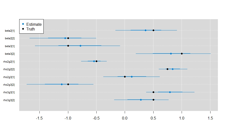
mcmcplots::caterplot(
  m1, reorder = FALSE
)
# and overlay the true simualted values
points(x = unlist(my_params), y = rev(1:10), pch = 19)
legend("topleft",
       c("Estimate", "Truth"),
       pch = 19,
       col = c(mcmcplots::mcmcplotsPalette(1), "black")
)

And it looks like the model did a sufficient job estimating the parameter values.

comparison of true parameter values to estimated. All true values fall within the 95% credible interval of each estimte.

Plotting out the results from your model

It’s a little more difficult to generate predictions with this model, as you need to do it for all of your linear predictors and then apply softmax to them. The code I have below here is not the fastest way to make these predictions, but I do think it’s written in a way that makes it a little easier to understand what is going on.

# Plot out some of the results.
#  make a design matrix with the covariate
#  you want to predict with. 
for_pred <- cbind(1, seq(-2,2, 0.05))

# get mcmc 
my_mcmc <- do.call("rbind", m1$mcmc)

# calculate latent state linear predictors/
#  grab is a utility function I put together
#  it's in ./R/functions/simulate.R. It just
#  pulls out the columns of a given linear
#  predictor with regex.
tmp1 <- for_pred %*% t(grab(my_mcmc, "beta2"))
tmp2 <- for_pred %*% t(grab(my_mcmc, "beta3"))

psi_preds <- list(
  state1 = matrix(NA, ncol = 3, nrow = nrow(for_pred)),
  state2 = matrix(NA, ncol = 3, nrow = nrow(for_pred)),
  state3 = matrix(NA, ncol = 3, nrow = nrow(for_pred)),
  marginal_occupancy = matrix(NA, ncol = 3, nrow = nrow(for_pred)),
  cond_breeding = matrix(NA, ncol = 3, nrow = nrow(for_pred))
)
# could write in a way to do this faster,
#  but this is easier to read.
pb <- txtProgressBar(max = nrow(for_pred))
for(i in 1:nrow(for_pred)){
  setTxtProgressBar(pb, i)
  tmp_pred <- t(
    apply(
      cbind(0, tmp1[i,], tmp2[i,]),
      1,
      softmax
    )
  )
  # marginal occupancy
  marg_occ <- tmp_pred[,2] + tmp_pred[,3]
  cond_occ <- tmp_pred[,3] / marg_occ
  # calculate quantiles of the 3 states
  tmp_pred <- apply(
    tmp_pred,
    2,
    quantile, 
    probs = c(0.025,0.5,0.975)
  )
  psi_preds$state1[i,] <- tmp_pred[,1]
  psi_preds$state2[i,] <- tmp_pred[,2]
  psi_preds$state3[i,] <- tmp_pred[,3]
  psi_preds$marginal_occupancy[i,] <- quantile(
    marg_occ,
    probs = c(0.025,0.5,0.975)
  )
  psi_preds$cond_breeding[i,] <- quantile(
    cond_occ,
    probs = c(0.025,0.5,0.975)
  )
}

# plot it out

plot(
  1~1, 
  type = "n", 
  xlim = c(-2,2),
  ylim = c(0,1),
  xlab = "Environmental covariate",
  ylab = "Occupancy probability",
  bty = "l",
  las = 1,
  cex.lab = 1.5
)
# 95% CI for state 2
polygon(
  x = c(for_pred[,2], rev(for_pred[,2])),
  y = c(psi_preds$state2[,1], rev(psi_preds$state2[,3])),
  col = scales::alpha("purple", 0.5),
  border = NA
)
# 95% CI for state 3
polygon(
  x = c(for_pred[,2], rev(for_pred[,2])),
  y = c(psi_preds$state3[,1], rev(psi_preds$state3[,3])),
  col = scales::alpha("gray50", 0.5),
  border = NA
)
# add median prediction
lines(
  x = for_pred[,2],
  y = psi_preds$state2[,2],
  lwd = 3,
  col = "purple"
)

lines(
  x = for_pred[,2],
  y = psi_preds$state3[,2],
  lwd = 3,
  lty = 3,
  col = "black"
)

legend(
  "topright",
  legend = c(
    "E(Owls present, no breeding)",
    "95% CI Owls present, no breeding",
    "E(Owls present, breeding)",
    "95% CI Owls present, breeding"
  ),
  fill = c(
    NA,
    scales::alpha("purple", 0.5),
    NA,
    scales::alpha("gray50", 0.5)
    ),
  border = c(NA, "black", NA, "black"),
  lty = c(1, NA, 3, NA),
  lwd = 3,
  col = c("purple", NA, "black", NA),
  bty = "n",
  cex = 1.2,
  seg.len = 1.5,
  x.intersp = c(2.2,1,2.2,1)
)

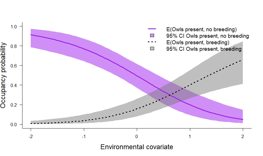
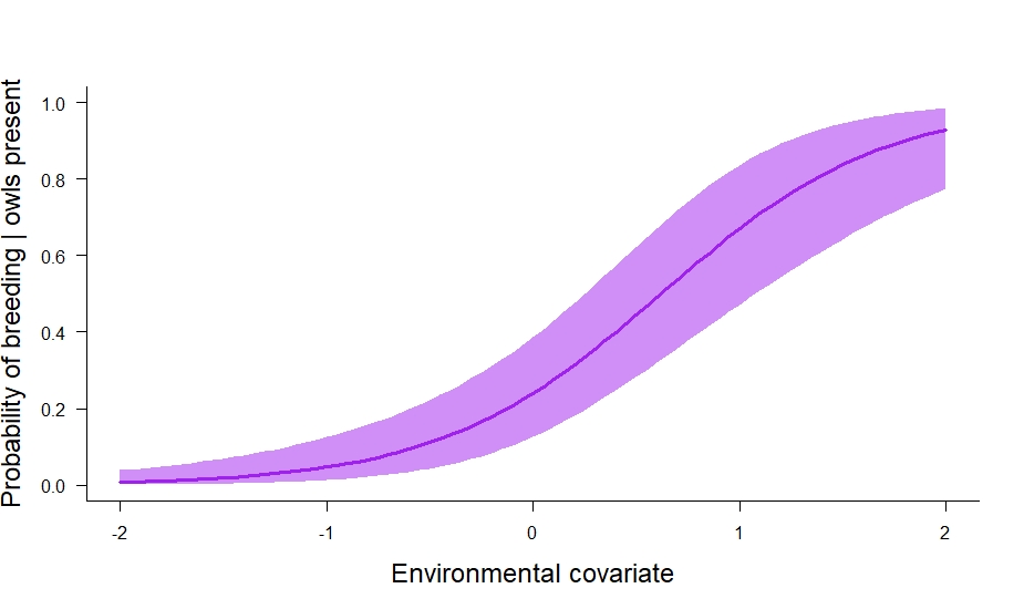
The occupancy probability of owls that do not breed is highest at low levels of this environmental covariate while the occupancy probability of owls that do breed is highest at high levels of this environmental covariate.

In the code above we also calculated the marginal occupancy probability (\(\psi_s^2 + \psi_s^3\)) and the conditional probability that owls breed given their presence (\(\frac{\psi_s^3}{\psi_s^2 + \psi_s^3}\)). I think the conditional probability is especially useful. In this particular case, it tells us about where owls breed relative to their underlying distribution. We can plot it out like so:

# plot out conditional probability of breeding | presence.

plot(
  1~1, 
  type = "n", 
  xlim = c(-2,2),
  ylim = c(0,1),
  xlab = "Environmental covariate",
  ylab = "Probability of breeding | owls present",
  bty = "l",
  las = 1,
  cex.lab = 1.5
)
# 95% CI for state 2
polygon(
  x = c(for_pred[,2], rev(for_pred[,2])),
  y = c(psi_preds$cond_breeding[,1], rev(psi_preds$cond_breeding[,3])),
  col = scales::alpha("purple", 0.5),
  border = NA
)

# add median prediction
lines(
  x = for_pred[,2],
  y = psi_preds$cond_breeding[,2],
  lwd = 3,
  col = "purple"
)

The conditional probability owls breed given their presence, it's highest at positive values of the environmental covariate.

And that is how to fit a static multistate occupancy model in JAGS. In future posts, I’ll cover autologistic and dynamic multistate models, and then probably move on to multistate models for multiple species (e.g., estimate statistical interactions among species).

Written on August 30, 2021