Mason Fidino

Species distribution models (SDMs) are useful tools in ecology and conservation biology. As the name implies, SDMs are used to estimate species presence or abundance across geographic space and through time. At their core, SDMs are a way to correlate environmental covariates–be they spatial, temporal, or both–to known locations of a species. Generally this is done through some form of regression analysis.

SDMs are being regularly improved, and one class of model I am very excited about is integrated SDMs. These models were developed, in part, to take advantage of the ever growing data sources that ecologists have access to (e.g., data from public participatory science, museum collections, and wildlife surveys, among others). What is great about integrated SDMs is that they allow you to combine these different types of species location data within the same statistical model. And because of this, integrated SDMs usually (not always) improve the predictive accuracy and precision of your model estimates. And while models that combine data sources are being used now more than ever, I would argue that they are still not seeing widespread use. So why is that?

In my opinion, the biggest hurdle that prevents the wide scale adoption of integrated SDMs is that the math associated to them can be complex and use non-standard likelihood functions that may need to be coded up from scratch. And to be honest, trying to understand that math is hard, especially as papers that introduce such models may need to skip some algebraic steps in the model formulation to save space! And while I am no expert in integrated SDMs, I wanted to take the time to dispel some of the confusion for one model I have been using in my own research, which is an integrated SDM that combines opportunistic presence-only data (e.g., data from public participatory science) with detection / non-detection data (e.g., data from camera traps, repeated bird counts, etc.).

In this post I am going to 1) walk through the model in Koshkina et al. (2017), 2) show how the model can be written out in JAGS, and 3) simulate some data and fit the model to show that it works. This post is long, so I have not included any of the simulation code here. Instead, you can find all of it, including the JAGS implementation of the model, on this GitHub repository. David Hope was also nice enough to implement this integrated model in Stan, and compared the parameter estimates from JAGS and Stan on their GitHub repository. So if you’re looking for a Stan implementation, look no further!

Here are some links to these three sections of the post in case you want to skip around.

1. The model
2. How to code up the model in JAGS
3. Share the results from simulated data fit to the model

The model

The Koshkina et al. (2017) integrated SDM, which was based on the model in Dorazio (2014), uses an inhomogeneous Poisson process model for the latent state. A Poisson process is just a mathematical object (e.g., a square with an x and y axis) in which points are randomly located. An inhomogeneous Poisson process, however, means the density of points on this object depends on your location on the object. Ecologically, this means that there is some region in geographic space (e.g., the city of Chicago, Illinois) and the modeled species abundance in that region varies across space.

So, for our region, B, we have a set of locations that individuals of our species occupies \(s_1,...,s_n\) and those locations are assumed to be a inhomogenous Poisson process. Thus, the limiting expected density of our species (number of individuals per unit area) can be described by the non-negative intensity function \(\lambda(s)\). Taking this one step further, the abundance of our species in region B is a Poisson random variable with mean:

which just means we take the integral across our landscape (i.e., slice up the landscape into tiny little bits, count all the individuals in each slice, and add that all together). It’s not difficult to make \(\lambda(s)\) a function of environmental variables, you use the log link and add in an intercept and slope term for each covariate \(\boldsymbol{x}(s)\). The fact that \(\boldsymbol{x}(s)\) is bold means that there are a vector of covariates for each location, and the first element of \(\boldsymbol{x}(s)\) should be a 1 so that the intercept is always included. For example, if you have 3 covariates \(\boldsymbol{x}(s)\) would actually have a length of 4. Thus, for i in 1,…,I covariates

The abundance model across the whole study area is then

Some other important things to note here is that we can also model the number of individuals within any subregion of B, which also has a Poisson distribution. So, if you have a set of non-overlapping subregions where \(r_1 \cup \cdots \cup r_k = B\) (this means the union of all the subregions equals B) then \(N(r_k) \sim \text{Poisson}(\mu(r_k))\).

I bring up this subregion modeling for two reasons. First, when we write the model in JAGS we are going to have to discretize the landscape to approximate the integral in the latent state model. So, we may as well start thinking about what breaking up the region into little pieces looks like now. Second, creating subregions makes it more intuitive to think about modeling occupancy instead of abundance. Why? Because if we set out to study a species in an area, chances are we know a priori that the probability at least one individual occupies B is 1, but there may be variation in the different subregions. To model occupancy we need to convert \(\mu(r_k)\) into a probability, which can be done with the inverse complimentary log-log link (inverse cloglog)

where \(\psi_k\) is the probability of occupancy for subregion \(r_k\). This could then be modeled as a Bernoulli trial where \(z_k = 1\) if the species occupies subregion \(r_k\).

And that is the latent state model! So far this should mostly remind you of Poisson regression (except for that little jaunt into occupancy modeling). The big exception, however, is that integral across space that we need to contend with in JAGS, and we’ll get there soon enough.

Because we are fitting a Bayesian model, we get to take a small departure from the way the data model is described in Koshkina et al. (2017). In their model explanation, they initially combined the presence-only data detectability and probability of detection from the detection/non-detection data into one term. We, however, will keep them separate the whole time. The detection / non-detection data model is the easier of the two, because it’s equivalent to the detection process of a standard occupancy model, so let’s start there.

Remember those \(r_k\) subregions of B that are non-overlapping parts of the study area? Let’s assume we do not sample every point in B and instead sample some subset of the subregions. For j in 1,…,J subregions sampled (hereafter sites) let \(r_k[j]\) represent the jth site sampled (\(k[j]\) means there is nested indexing). We then have for w in 1,..,W sampling occasions at these sites, which results in a J by W binary observation matrix \(y_{j,w}\). If we detected the species at site j on sampling occasion w, \(y_{j,w} = 1\), otherwise it is zero (assuming equal sampling at all sites). The probability of detecting the species given their presence \(\rho_{j,w}\) can then be estimated as:

and \(\rho_{j,w}\) can be made a function of covariates using the logit link, which could vary across sites or sampling occasions. For q in 1,…,Q covariates this is the linear predictor of the detection / non-detection data model is

where a is a vector of regression coefficients (intercept and slope terms) and V is a Q by J by W array where the first element of \(\boldsymbol{v}_{j,w} = 1\) to account for the model intercept.

Modeling the opportunistic presence-only data is a little more complex because we assume the presence-only data are a thinned Poisson process. What that means is that we multiply \(\lambda(s)\) by some estimated probability (i.e., the presence-only detectabilty), which “thins” it. This thinning is helpful because we expect that the opportunistic presence-only data has some bias in where it was collected becuase there may not be a rigorous sampling design. As such, some areas may be oversampled while other areas are undersampled and we do not want that to bias our species abundance estimate.

The probability of being detected in the presence-only data, b(s), can be made a function of g in 1,..,G covariates such that

Where \(\boldsymbol(c)\) is a vector that contains the intercept and slope terms while \(\boldsymbol(h)(s)\) is a vector of G covariates, where the first element is 1 to account for the intercept Before we move on there is one really important thing to bring up. For this model to be identifiable, \(\boldsymbol{x}\)(s) must have one unique covariate that \(\boldsymbol{h}(s)\) does not have, and \(\boldsymbol{h}(s)\) must have one unique covariate \(\boldsymbol{x}(s)\) does not have. If you put the exact same covariates on the latent state and the presence-only data model, your model will not converge. Keep that in mind while you consider hypotheses for your own data!

As this is a thinned Poisson process, the the expected number of presence only locations throughout B is the product of \(\lambda(s)\) and\(b(s)\), assuming that the species was detected at m locations \(s_1,\cdots,s_m\) where m < n. In other words, we make the assumption that the number of individuals detected in the presence-only data is less than the total number of individuals of that species on the landscape. Thus,

Following Dorazio (2014) the likelihood of the presence only data is

And if I had to guess, this is where people can get lost with this model! This likelihood is not necessarily that intuitive so it makes it difficult to know how to code it in your Bayesian programming language of choice. But if we go through it piece by piece, the math here is not all that scary.

To let you know we are headed, this equation is dividing the thinned Poisson process at all of the presence only data points by the thinned Poisson process over the entire region B (i.e., the integral). Yet, there is no fraction here, so how did I arrive at this conclusion? Whenever you see negative signs thrown around with exponential terms or natural logarithms, there could be some divison happening on the log scale. For example, if you remember that exp(log(x)) = x, here are two different ways to write the equation \(10 / 2 = 5\)

This is also really easy to check in R as well

10 / 2
[1] 5

exp(log(10) - log(2))
[1] 5

exp(-log(2)) * 10
[1] 5

If you look closely at that third example, its not too hard to recognize it as a simplified version of \(\text{exp} \big(- \int_B\lambda(s)b(s)ds \big) \prod_{i=1}^m\lambda(s_i)b(s_i)\). So, because exp(-x) * y == y/x, the first term term in our likelihood is the denominator and represents the thinned Poisson process over the region B, while the second term in our likelihood is the numerator that represents the thinned Poisson process over the m presence-only locations. With that out of the way, we just need to figure out what the likelihood is doing with the regression coefficients from the latent state model (\(\beta\)) and the regression coefficients associated to the presence-only thinning probability (\(\boldsymbol{c}\)).

For those familiar with logistic regression, you can hopefully notice that the likelihood

made a slight modification to the inverse logit link, \(\text{logit}^{-1}(x) = \frac{\text{exp}(x)}{1 + \text{exp}(x)}\). The inverse logit link is important to know, especially if you do any amount of occupancy modeling, because it converts logit-scale coefficients back to the probability scale. It looks like this likelihood function added the log-scale coefficients from the latent state model (\(\boldsymbol{\beta}\)) into the numerator of the inverse logit link, while the logit-scale coefficients (\(\boldsymbol{c}\)) from the thinning process are in the numerator and the denominator. To see what this means, let’s explore how this modified inverse logit link function works in R, assuming that \(\lambda(s) = 20\) and \(b(s) = 0.75\).

# The parameters
lambda <- 20
b <- 0.75

# Transform these variables to their
#  respective scales. 

# Log link for lambda_s
log_lambda <- log(lambda)

# logit link for b_s
logit_b <- log(b/(1 - b)) 

# Modified inverse logit
answer <- exp(log_lambda + logit_b) / (1 + exp(logit_b))

# compare that to lambda * b
#  both == 15
c(answer, lambda * b)
[1] 15 15

Therefore, this modified inverse logit is the inverse link function for the regression coefficients associated to the thinned Poisson process \(\lambda(s)b(s)\)! Knowing that, we could take the presence-only data likelihood and abstract it out a little further:

where

And that is the breakdown of the likelihood of the presence-only data. Hopefully this additional explanation here makes the model a bit easier to understand. In summary, this model has three linear predictors. One for the latent state that is partially informed by the presence-only data and detection/non-detection data, one to account for the bias in the opportunistic presence-only data, and one to account for false absences in the detection / non-detection data.

Back to top ⤒

How to code up the model in JAGS

For this example I’m going to focus on modeling species occupancy instead of abundance, though the model can easily be modified to estimate abundance by changing the likelihood function of the latent state model.

To code up this model in JAGS there are two things we need to overcome.

1. Approximating the integrals in the model with a Riemann sum.
2. Incorporate the non-standard likelihood of the presence-only data model with the Bernoulli “ones trick”.

The first step is not difficult. For the region B, all we need to do is break it up into a “sufficiently fine grid” (Dorazio 2014) and evaluate the model in each grid cell.

What is sufficiently fine? I’ve seen some suggestions that you need at least 10000, but in reality the number of cells is going to depend on the landscape heterogeneity you are trying to capture and your data. For example, a small study region roughly the size of a city may not need 10000 grid cells. In my own research, I’ve had success splitting Chicago, IL, which is about 606 km², into roughly 2500 500m² grid cells (and the simulation below has around 4500 grid cells). So if you are trying to use this model on your own you may need to do some trial and error to determine what is an appropriate cell count is (i.e., fit the model with different grid cell sizes to see if it has an influence on the parameters in the latent state model).

Perhaps the trickiest part related to discretizing the region, however, means all of the data input into the model needs to be aggregated to the scale of the grid (i.e., the covariates and species data). In R, the raster::aggregate function will do most of that work for you. In the simulated example, I also created the function agg_pres() which aggregated species presence on the landscape to the appropriate grid size (which is in the script ./utilities/sim_utility.R here).

Now back to the model. Let npixel be the total number of grid cells on our landscape and cell_area be the log area of the gridded cell (we have to include a log offset term into the latent state linear predictor to account for the the gridding we did). The latent state model is then:

for(pixel in 1:npixel){
	# latent state linear predictor
	#
	# x_s  = covariates for latent state
	# beta = latent state regression coefficients
	# cell_area = log area of grid cell 
	#
	log(lambda[pixel]) <-inprod(x_s[pixel,1:I], beta[1:I]) + cell_area
	# Species presence in a gridcell as a Bernoulli trial
	z[pixel] ~ dbern(1 - exp(-lambda[pixel]))
}

Remember, however, that the presence-only data model needs to be evaluated across the entire landscape as well (i.e., the integral that is the denominator of the presence-only data model likelihood). Therefore, we should also calculate the thinning probability for each cell here too.

for(pixel in 1:npixel){
	# latent state linear predictor
	#
	# x_s  = covariates for latent state
	# beta = latent state model regression coefficients
	# cell_area = log area of grid cell 
	#
	log(lambda[pixel]) <-inprod(x_s[pixel,], beta) + cell_area
	# Species presence in a gridcell as a Bernoulli trial
	z[pixel] ~ dbern(1 - exp(-lambda[pixel]))
	# presence only thinning prob linear predictor
	#
	# h_s = covariates for thinning probability
	# cc  = presence-only data model regression coefficients
	#
	logit(b[pixel]) <-  inprod(h_s[pixel,] , cc)
}

And now we can start coding up the likelihood of the presence-only data model. While you can easily create your own likelihood functions in Nimble, it’s not quite as simple in JAGS. However, there are some workarounds, and my personal favorite is the Bernoulli “ones trick”.

To do this for the presence-only data model there are a two steps. First, code up the likelihood for each of the m presence-only data points. Second, input that likelihood for each data point into a Bernoulli trial and divide it by some large constant value to ensure the likelihood is between 0 and 1 such that ones[i] ~ dbern(likelihood[i]/CONSTANT), where ones is a vector of ones the same length as m. CONSTANT = 10000 is a good place to start. This little trick evaluates the likelihood of data point i given the current model parameters in the MCMC chain, which is exactly what we need.

Note, however, that the presence-only data model likelihood function presented in Koshkina et al. (2017) is for ALL the data points, and we need to evaluate the likelihood of each data point on its own. To do this, all we need to do is remove the product from the numerator because we are only looking at a single data point from the numerator and divide the denominator by m (i.e., the number of presence-only data points). If you recall that exp(log(x) - log(y)) = x/y we can write the presence-only likelihood in JAGS using nested indexing to map the m datapoints back to their respective grid cell. If I wanted to I could have coded up the presence-only data model inverse link function and applied it to the regression coefficients & covariates for each cell. However, we have already calculated lambda and b in the model so we can use them instead.

# The presence only data model.
#
# This part of the model uses
#  what we have calculated above (lambda
#  and b). The denominator of this likelihood
#  is a scalar so we can calculate it
#  outside of a for loop. Let's do that first,
#  which we are approximating as a Riemann sum.
#
po_denominator <- inprod(lambda[1:npixel], b[1:npixel] ) / m
#
# Loop through each presence-only datapoint
#  using Bernoulli one's trick. The numerator
#  is just the thinned poisson process for
#  the ith data point, and we use some
#  nested indexing to map the data to 
#  it's associated grid cell.
for(po in 1:m){
  ones[po] ~ dbern(
  	exp(
  	  log(lambda[po_pixel[po]]*b[po_pixel[po]]) -
  	  log(po_denominator)
	) / CONSTANT
  )
} 

Here, po_pixel denotes the grid cell of the ith presence only data point.

Finally, the detection/non-detection data model is basically what you’d see in a standard occupancy model, but again uses nested indexing to map the sampled site to it’s respective grid cell. I’m making the assumption here that the W sampling occasions are i.i.d. random variables and so will model them as a binomial process such that

for(site in 1:nsite){
  # detection/non-detection data model linear predictor
  #
  #  v = detection covariates for the entire region B
  #  a = det/non-det data model regression coefficients
  #
  logit(rho[site]) <-inprod(v[pa_pixel[site], ],a)
  # The number of detections for site is a binomial
  #  process with Pr(rho[site]) | z = 1 with
  #  W sampling occasions per site.
  y[site] ~ dbin(
    z[pa_pixel[site]] * rho[site],
    W
  )
}

Here is all of the model put together plus some non-informative priors for all the parameters and a derived parameter to track how many cells the species occupies.

model{
  # Bayesian version of the Koshkina (2017) model.
  #
  # The latent-state model
  for(pixel in 1:npixel){
    # latent state linear predictor
    #
    # x_s  = covariates for latent state
    # beta = latent state model regression coefficients
    # cell_area = log area of grid cell 
    #
    log(lambda[pixel]) <-inprod(x_s[pixel,], beta) + cell_area
    # Species presence in a gridcell as a Bernoulli trial
    z[pixel] ~ dbern(1 - exp(-lambda[pixel]))
    # presence only thinning prob linear predictor
    #
    # h_s = covariates for thinning probability
    # cc  = presence-only data model regression coefficients
    #
    logit(b[pixel]) <-  inprod(h_s[pixel,] , cc)
  }
  # The presence only data model.
  #
  # This part of the model just uses the
  #  what we have calculated above (lambda
  #  and b). The denominator of this likelihood
  #  is actually a scalar so we can calculate it
  #  outside of a for loop. Let's do that first.
  #
  # The presence_only data model denominator, which
  #  is the thinned poisson process across the
  #  whole region (divided by the total number of 
  #  data points because it has to be 
  #  evaluated for each data point).
  po_denominator <- inprod(lambda[1:npixel], b[1:npixel] ) / m
  #
  # Loop through each presence-only datapoint
  #  using Bernoulli one's trick. The numerator
  #  is just the thinned poisson process for
  #  the ith data point.
  for(po in 1:m){
    ones[po] ~ dbern(
      exp(
        log(lambda[po_pixel[po]]*b[po_pixel[po]]) -
          log(po_denominator)
      ) / CONSTANT
    )
  } 
#
# Detection / non-detection data model
for(site in 1:nsite){
  # detection/non-detection data model linear predictor
  #
  #  v = detection covariates for the entire region B
  #  a = det/non-det data model regression coefficients
  #
  logit(rho[site]) <-inprod(v[pa_pixel[site], ],a)
  # The number of detections for site is a binomial
  #  process with Pr(rho[site]) | z = 1 with
  #  W sampling occasions per site.
  y[site] ~ dbin(
    z[pa_pixel[site]] * rho[site],
    W
  )
}
#
# Priors for latent state model
for(latent in 1:nlatent){
  beta[latent] ~ dnorm(0, 0.01)
}
# Priors for presence-only data model
for(po in 1:npar_po){
  cc[po] ~ dlogis(0, 1)
}
# Priors for det/non-det data model
for(pa in 1:npar_pa){
  a[pa] ~ dlogis(0, 1)
}
# Derived parameter, the number of cells occupied
zsum <- sum(z)
}

Back to top ⤒

Simulating some data

I’m not going to share all of the simulation code here as it is hundreds of lines long. However, I do want to demonstrate that this model works, and works better than a standard occupancy model. To look at all the simulation code and try it for yourself, visit this repository here. You just need to run through simulate_poisson_process.R to simulate the data and fit the models.

If you are not interested in that code, here are the steps I took to simulate the data:

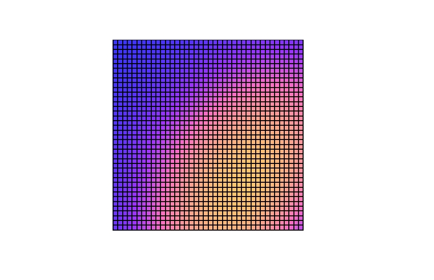
1. Create the study region and give it a spatially autocorrelated environmental covariate.
2. Generate latent species abundance on the landscape, which is correlated to the environmental covariate from step 1.
3. Create a secondary environmental covariate that is correlated to the bias in the presence-only data.
4. Generate presence-only data, which samples from the latent species abundance in step 2 based on the environmental covariate in step 3 (i.e., some individuals are observed in the presence-only dataset).
5. Aggregate covariates and species presence on the landscape down to a coarser resolution for modeling purposes.
6. Place some sites to sample your detection / non-detection data across the landscape at the same scale as this new coarser resolution.
7. If the species is present at these sites, sample their presence with imperfect detection.

Following this I fit the simulated data to two models. The first model had the same latent-state and detection/non-detection data model, but I removed the presence-only data model so that it is just a standard occupancy model with a cloglog link. The second model is the integrated model from above fit to all of the data.

For this simulation, I assumed there was a single covariate that influenced the latent state and one covariate that influenced the bias of the presence-only data. For simplicity, I also assumed that imperfect detection at sampling sites did not vary (i.e., the data model for detection/non-detection data was intercept only). Some other general bookkeeping for this simulation:

1. One hundred sites were sampled for the detection / non-detection data.
2. The intercept and slope coefficients for the latent state were respectively 6 and 1.
3. The intercept and slope coefficients for the presence-only thinning probability were respectively -0.75 and 1.5.
4. The by-survey probability fo detecting an individual given their presence at a sample site was 0.3 (about -0.85 on the logit scale).

When comparing the outputs of the latent state estimates from the standard occupancy model that only used detection / non-detection data to the integrated occupancy model that also used presence-only data, it clear that the integrated model has greater accuracy and precision.

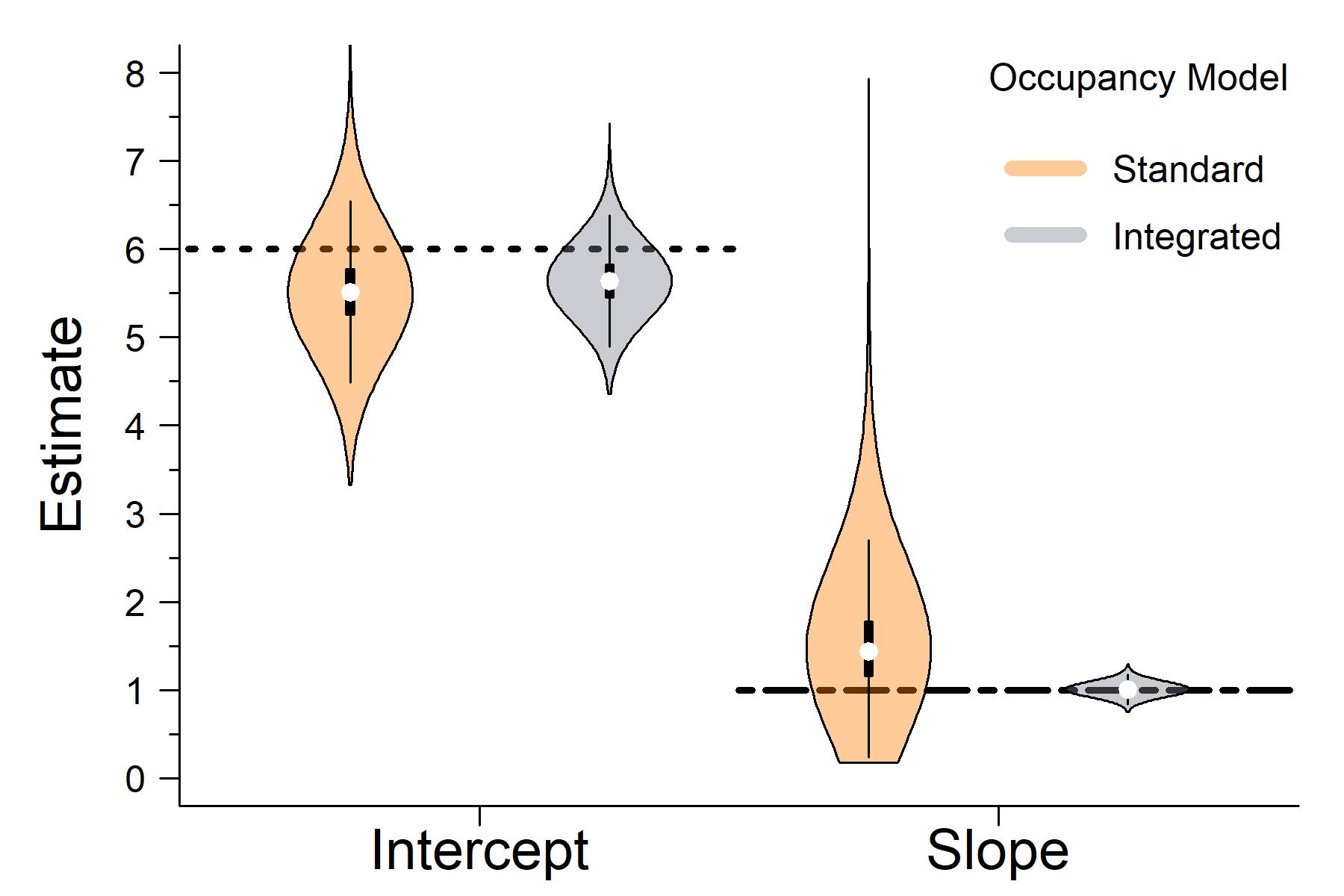
The horizontal lines in the plot above are the true parameter values I used to simulate the data..

Digging into the results from the rest of model, it’s also clear that the integrated model did a great job retrieving the parameters from the other linear predictors.

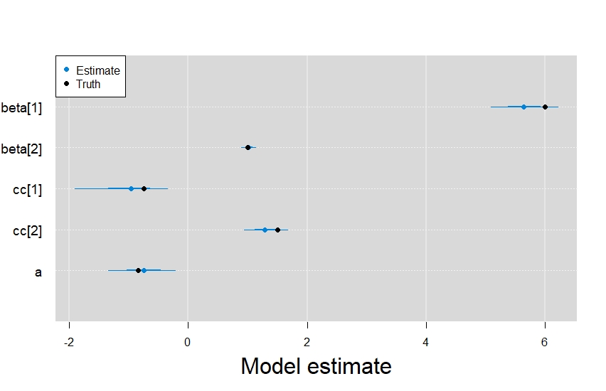
In order, beta represents the latent state terms, cc are the presence-only data model terms, and a was the intercept term from the detection/non-detection data model.

One last thing before I wrap this up. If you use this model yourself, you must remember to include the log-offset term in order to make model predictions. For example, if I wanted to make predictions across the environmental covariate that was related to the species latent occupancy state, the code would look something like (assuming you are working with the model objects from simulate_poisson_process.R:

# matrix for predictions.
#  intercept and slope.
for_pred <- cbind(1, seq(-2,2, 0.01))

# The log-offset I supplied to JAGS
my_log_offset <- my_data$cell_area

# get mcmc samples for latent state terms
#  intmm = integrated mcmc samples
latent_parms <- intmm[,c("beta[1]", "beta[2]")] 

# predictions on cloglog scale
my_preds <- latent_parms %*% t(for_pred) + my_log_offset

# inverse cloglog to convert to probability
my_preds <- 1 - exp(-exp(my_preds))

# get quantiles for plotting
my_preds <- apply(
  my_preds,
  2,
  quantile,
  probs = c(0.025,0.5,0.975)
)

plot(
  my_preds[2,] ~ for_pred[,2],
  type = "l",
  lwd = 3,
  ylim = c(0,1),
  xlab = "Environmental covariate",
  ylab = "Pr(Occupancy)",
  las = 1,
  bty = "l"
)
lines(my_preds[1,] ~ for_pred[,2],lty =2, lwd = 2)
lines(my_preds[3,] ~ for_pred[,2],lty =2, lwd = 2)

legend("topleft", c("Median estimate", "95% CI"), lty = c(1,2), lwd = c(3,2),
       bty = "n", cex = 1.3)

And there you have it, a JAGS implementation of the Koshkina et al. (2017) model.

Back to top ⤒