Mason Fidino

There are a lot of different ways to algebraically write out a statistical model, and as such there are an equally large number of ways to write a model in Nimble, JAGS, or Stan. One technique that I see in introductory text books on Bayesian Modeling is nested indexing, which is a way to map one part of a model to another through a vector of values. The most common way nested indexing is used is to include a random effect term in the linear predictor of a model. For example, for n in 1,…,N data points, and i in 1,…,I categories of a random effect term, the linear predictor of a random intercept model could be written as:

Where the \(i[n]\) is a vector of length N that denotes which category the nth data point belongs to. If we assume this is for logistic regression, this could be written in In JAGS as:

model{
	for(n in 1:N){
		logit(mu[n]) = beta0 + beta[re_vec[n]]
		y[n] ~ dbern(mu[n])
	}
	beta0 ~ dnorm(0, 0.01)
	for(i in 1:I){
		beta[i] ~ dnorm(0, tau)
	}
	sigma ~ Unif(0.001,1000)
	tau <- 1 / sqrt(sigma) 
}

where re_vec equals \(i[n]\), so it denotes the numeric category of the nth datapoint. Often times the categories you have in R are represented as factors, and making a numeric vector from a factor is very simple.

# The gl function is just a way to generate a bunch of levels
#  for a factor. You'd generally be applying `factor()` to
#  some character data in your own dataset.
example_data <- data.frame(
  categories = gl(10,10, labels = LETTERS[1:10])
)

example_data$categories
  [1] A A A A A A A A A A B B B B B B B B B B C C C C C C C C C C D D
 [33] D D D D D D D D E E E E E E E E E E F F F F F F F F F F G G G G
 [65] G G G G G G H H H H H H H H H H I I I I I I I I I I J J J J J J
 [97] J J J J
Levels: A B C D E F G H I J

Here, we have 10 categories, each represented with a letter (A through J). To make this numeric you simply convert your factor:

example_data$re_vec <- as.numeric(example_data$categories)

example_data$re_vec
  [1]  1  1  1  1  1  1  1  1  1  1  2  2  2  2  2  2  2  2  2  2  3
 [22]  3  3  3  3  3  3  3  3  3  4  4  4  4  4  4  4  4  4  4  5  5
 [43]  5  5  5  5  5  5  5  5  6  6  6  6  6  6  6  6  6  6  7  7  7
 [64]  7  7  7  7  7  7  7  8  8  8  8  8  8  8  8  8  8  9  9  9  9
 [85]  9  9  9  9  9  9 10 10 10 10 10 10 10 10 10 10

Here, re_vec (random effect vector) is of length 100, the first 10 values are 1 because they belong to the first cateogory, the 11th through 20th values are 2 because they belong to the second category, etc. etc.

And that is generally where nested indexing is left. You can use it as a way to specify random effects within a model, or other types of categorical variables. However, as nested indexing is literally just a way to map one piece of information to another, it can, and I think it should, be used way more broadly. Let me show you a couple of examples to demonstrate the power of nested indexing.

Example 1: Speeding up your model that has a lot of missing data.

For occupancy studies, often times sampling is not uniform across sites, such that the number of repeat visits varies. When there is not much missing data this may not be much of an issue, you simply fill the detection / non-detection matrix with NA values where you lack data. However, when working with very large data sets this can cause problems (e.g., lots of sites sampled, many repeat observations, or both). At best, the model compiles but takes much longer to run because of all the NA nodes it has to estimate. At worst, you may not have enough RAM to hold the model in your memory!

If you have a lot of missing data it may be simpler to model the detection non-detection data in long-format (or a ragged array). JAGS does not allow for ragged arrays, but you can mimic them with the use of nested indexing! So, let’s simulate some data, throw some of it out, and demonstrate how to use nested indexing to skip over all of those pesky NA values you generally do not need to evaluate in an occupancy model. The next code block is a lot of the general data simulation, up to the point where we input a bunch of missing data into the detection / non-detection matrix.

# Load some libraries we'll need
library(runjags)
library(mcmcplots)

# Step 1. Simulate some occupancy data

set.seed(-132)

# number of sites and repeat surveys
# We are using LOTS of sites here, as this is where
# nested indexing comes in really useful.
nsite <- 500
nrep <- 20

# design matrix for occupancy
X_occupancy <- cbind(
  1,
  rnorm(nsite)
)

# occupancy parameters, intercept and slope
b_occupancy <- c(
  0.73,
  -1
)

# log-odds of occupancy
logit_prob_occupancy <- X_occupancy %*% b_occupancy

# convert to probability
prob_occupancy <- plogis(
  logit_prob_occupancy
)

# True occurence
z <- rbinom(
  nsite,
  1,
  prob_occupancy
)

# Step 2. Add imperfect detection

# design matrix for detection. Assuming
#  that there are observation specific
#  covariates. Site x n parameter x repeat visits
X_detection <- array(
  rnorm(nsite*2*nrep),
  dim = c(nsite, 2, nrep)
)

# convert the first column to 1's for the intercept
X_detection[,1,] <- 1

# detection parameters, intercept and slope
b_detection <- c(
  1,
  -0.5
)

# log odds of detection
logit_prob_detection <- apply(
  X_detection,
  3,
  function(x) x %*% b_detection
)


# probability of detection
prob_detection <- plogis(
  logit_prob_detection
)

# simulate the detection/ non-detection data
y <- matrix(
  rbinom(
    nsite*nrep,
    1,
    sweep(prob_detection, 1, z, "*")
  ),
  ncol = nrep,
  nrow = nsite
)

# Step 3. Lose some of the data. Here we are going to
#  assume that sampling is unequal across sites, and therefore
#  each site will have a different number of repeat visits.
#  We are going to simualte the number of samples per site
#  and then randomly input NA's into the y matrix.
samps_per_site <- sample(
  5:nrep,
  nsite,
  replace = TRUE
)

# just going to loop through and input NA's
y_na <- y
for(i in 1:nsite){
  to_na <- sample(
    1:nrep,
    nrep - samps_per_site[i],
    replace = FALSE
  )
  y_na[i, to_na] <- NA
}

# Check out many NA values there are
sum(is.na(y_na))/length(y_na)

So through this simulation, almost 40% of the detection/non-detection matrix we would supply to JAGS is full of NA values. In this case, that is nearly 4000 elements that JAGS would need to estimate during each step of an MCMC chain that is does not need to! So, now comes the complicated part. To use nested indexing, we need to go from wide format to long format with the detection / non-detection data. To do so, we use which() and set arr.ind = TRUE, which can be used to identify where there are non NA values in the detection / non-detection matrix.

# Step 4. Determine where we have data.
#  If we just used y, we would be inputting a nsite*nrep
#  matrix with a LOT of NA's. We can reduce this.
#  As a reminder, sites are along rows and 
#  secondary observations are along columns.
has_data <- which(
  !is.na(y_na),
  arr.ind = TRUE
)

# Because the row ID tells us which site we have,
#   and the col ID tells us which observation. We
#   can use this information to collect the
#   appropriate observation covariates

# ob cov long will hold the covariate values for each
#  observation that we have data in long format. This
#  will be number of observations long and 2 columns 
#  wide (one for the interecpt and one for the continuous
#  covariate on detection that varies with each
#  secondary observation).
ob_cov_long <- matrix(
  1,
  nrow(has_data),
  ncol = 2
)

# Loop thorugh the data and collect
#  the appropriate covariates.
for(i in 1:nrow(has_data)){
  ob_cov_long[i,2] <- X_detection[
    has_data[i,1],
    2,
    has_data[i,2]
    ]
}

# We need to make the detection matrix long format as well.
#   We need this to have the same ordering as has_data.
#   This is actually really simple to do, we just remove
#   all the NA values and convert it to a vector like so.
y_long <- y_na[!is.na(y_na)]

# Finally, combine all the necessary data into a list for JAGS
# set up data list
data_list <- list(
  y = y_long,
  site_id = has_data[,1], # Indexes which site
  X_occ = X_occupancy,
  X_det = ob_cov_long,
  nsite = nsite,
  nvisits = length(y_long)
)

To wrap up this part of the simulation we just need to bag up all of the data for JAGS in a list. One important thing to note is that because we have specified the detection data in long-format, all we need to do for nested indexing is map the latent state model (500 sites) to the detection model (6102 detections) with a single vector that denotes what site a given detection is associated to, which we will call site_id in the model, and it is represented in this case as the first column of the has_data matrix we generated.

data_list <- list(
  y = y_long,
  site_id = has_data[,1],  
  X_occ = X_occupancy,
  X_det = ob_cov_long,
  nsite = nsite,
  nvisits = length(y_long)
)

The occupancy model itself is very close to a standard occupancy model and can be found here. The only important difference is the nested indexing we used in the detection model.

model{
  # priors
  B_occ[1] ~ dlogis(0,1)
  B_occ[2] ~ dlogis(0,1)
  B_det[1] ~ dlogis(0,1)
  B_det[2] ~ dlogis(0,1)
  # latent state model
  for(i in 1:nsite){
    logit(psi[i]) <- inprod(B_occ, X_occ[i,])
    z[i] ~ dbern(psi[i])
  }
  # detection model, the important part
  #  is just indexing what site the jth data point
  #  is associated to via z[site_id[j]].
  for(j in 1:nvisits){
    logit(rho[j]) <- inprod(B_det, X_det[j,])
    y[j] ~ dbern(rho[j] * z[site_id[j]])
  }
}

Here is the rest of the code to fit the model.

# getting some initial values for z,
#  equals 1 if we detected it, 
#  otherwise it is 0.

z_init <- rowSums(y_na, na.rm = TRUE)
z_init[z_init > 1] <- 1

my_inits <- function(chain){
  gen_list <- function(chain = chain){
    list(
      z = z_init,
      B_occ = rnorm(2),
      B_det = rnorm(2),

      .RNG.name = switch(chain,
        "1" = "base::Wichmann-Hill",
        "2" = "base::Wichmann-Hill",
        "3" = "base::Super-Duper",
        "4" = "base::Mersenne-Twister",
        "5" = "base::Wichmann-Hill",
        "6" = "base::Marsaglia-Multicarry",
        "7" = "base::Super-Duper",
        "8" = "base::Mersenne-Twister"
      ),
      .RNG.seed = sample(1:1e+06, 1)
		)
	}
	return(switch(chain,
		"1" = gen_list(chain),
		"2" = gen_list(chain),
		"3" = gen_list(chain),
		"4" = gen_list(chain),
		"5" = gen_list(chain),
		"6" = gen_list(chain),
		"7" = gen_list(chain),
		"8" = gen_list(chain)
	)
	)
}

m1 <- run.jags(
  model = "ragged_occupancy.R",
  data = data_list,
  n.chains = 3,
  monitor = c("B_occ", "B_det"),
  adapt = 1000,
  burnin = 2000,
  sample = 5000,
  thin = 1,
  inits = my_inits,
 modules = "glm",
 method = "parallel"
)

And plotting out the results shows that the nested indexing approach still returns the correct parameter estimates.

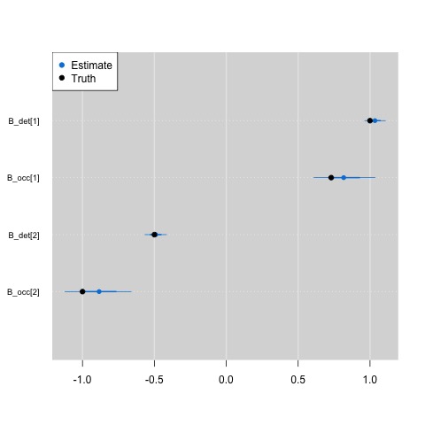
In my experience, I deal with missing data often, especially when modeling data across the Urban Wildlife Information Network (UWIN), and so knowing that this model is equivalent to a standard occupancy model is great. For example, I made heavy use of nested indexing for the analysis of this paper here, where we fit a multi-region occupancy model to data from 20 partnering UWIN cities.

Example 2: Linking different models to your occupancy model to address new ecological questions.

This post is already long, so I’ll keep this bit short, but one aspect of nested indexing that I have gotten really interested in over the last few years is to either use the same data source in different ways within your occupancy model, or to combine different data sources entirely. For example, a lot of my own research is done with camera trapping, and often enough we discretize the photo detections of species down to some secondary sampling period (e.g., days or weeks). However, the photos may also house more information than just what species is present. As just one example, in this paper we modeled the distribution of coyote (Canis latrans) as well as the distribution of mangy coyote throughout Chicago, IL. To do so, we had to go back through all of our coyote images to identify which coyote had visible signs of mange. Following this, I developed a multi-state occupancy model that accounts for by-site false absences of coyote and also by-image false absences of detecting mange in a coyote photo. We found that it was far easier to detect mange on a coyote image if the photo was clear, during the daytime, and had atleast half of the coyote in the image. The paper (you can find a pdf on my publications page) goes through the math behind this, and all of the results, so I am not going to cover it here. If you want a simualted example of the model, which most assuredly has some nested indexing, look no further than the supplemental material.

So, if you are collecting camera trap data, start thinking about how you can take advantange of nested indexing to answer different ecological questions! And while I didn’t get to this here, in a future post I’ll show how you can use nested indexing to map data to one another in an integrated occupancy model.