The normal distribution
Regression analysis can be used to estimate the relationship between different variables. To better understand regression analysis, I think it is important to learn about some standard probability distributions that are used to fit different types of models to data. Without getting too technical, probability distributions are mathematical functions that provide the probability of different outcomes of an experiment, and we use these standard distributions because they have proven to be helpful. Probability distributions have parameters, which are numeric inputs, that alter how likely different outcomes are for a specific experiment. In the real world, we are generally interested in estimating what these parameters are from data.
Arguably, one of the best-known probability distributions is the normal distribution, which resembles a bell curve:
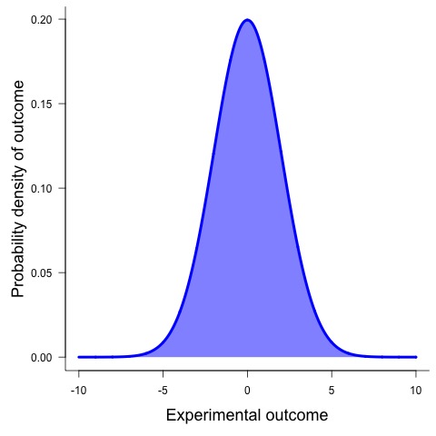
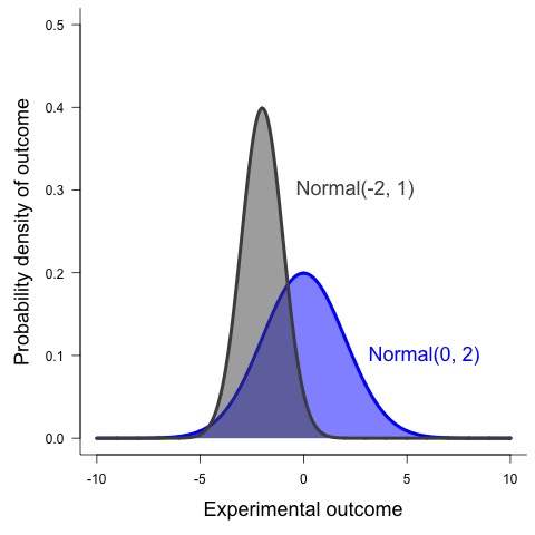
The normal distribution often follows the notation: \(Normal(\mu, \sigma)\). Lookinga at this we can see this distribution has two parameters, \(\mu\) and \(\sigma\), which respectively represent the population mean and standard deviation. In more general terms, \(\mu\) is a location parameter, which describes the mean, median, or mode of a statistical distribution while \(\sigma\) is a scale parameter. Scale parameters indicate the spread of a distribution and the larger the scale parameter the more spread out the distribution. In the plot above the most likely value is the mean, which is 0, while the standard deviation is 2. It is possible for \(\mu\) to be any number between \(-\infty\) and \(\infty\). Convserly, the scale parameter,\(\sigma\), must be greater than or equal to zero. By changing the location and scale the shape of the distribution changes.
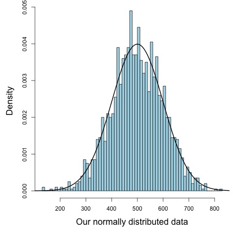
Because \(\mu\) can be any value value, data generated from a normal distribution can also take any value. If we wanted to randomly generate normally distributed data in R, we would use the function rnorm().
# generate 2000 random normal data points with mean = 500 and sd = 100.
our_normal_data <- rnorm(n = 2000, mean = 500, sd = 100)

# plot out the density of the data as a histogram
hist(our_normal_data,
     freq = FALSE,
     breaks = 50,
     col = 'lightblue',
     main = "",
     xlab = "Our normally distributed data")

# Calculate the probability density of a range of points from
#  0 to 1000 from Normal(mean = 500, sd = 100)
range_of_values <- seq(0,1000,1)
normal_density <- dnorm(range_of_values, mean = 500, sd = 100)

# add this to the histogram
lines(normal_density ~ range_of_values, lwd = 2)