A somewhat hacky solution to getting a progress bar when Bayesian fitting models in parallel with NIMBLE

Okay, so I’m finally starting to make the move from JAGS to NIMBLE. The reason I’ve decided to do this is mostly because of all the customization you can do with NIMBLE in terms of easily specifying different samplers. JAGS uses a slice sampler, which requires multiple proposals for each step of an MCMC chain. This often results in a great acceptance rate for proposals, but it takes longer than simpler samplers like a random walk metropolis (the default sampler for NIMBLE). As a result, models can take a loooonnnggg time to run in JAGS if you have a lot of data. Additionally, seeing a lot of active development with NIMBLE is great too, so I’m excited to give it a try.

However, if I’m being honest, what kept me coming back to JAGS over and over again was that running models in parallel is just not as easy in NIMBLE. In the former, it’s as simple as specifying it in an argument when you fit a model. For the latter, you’ve got to spin up a cluster on your computer and modify how you write your model. Doing this is not that difficult, and NIMBLE provides an example of how to do this too, which is great. However, by running models in parallel this way you essentially lose the ability to see a progress bar, which kind of sucks. A lot of the models I fit take days to run, and so knowing that they are slowly chugging along is helpful (especially when collaborators ask when I’ll have the results to share with them).

So, I hobbled together a little way to essentially get the progress bar back. However, what I am describing below is 100% a hacky solution to dealing with this, and probably only useful if you are fitting models that take a really long time to run. Regardless, I’m sharing it here just in case.

Give me back my progress bar

You can fit your NIMBLE model in parallel very similarly to the way you would do so normally, but there are a few key differences:

You have to send the script with the parallelized NIMBLE model to your command line, which means you need to be able to use the Rscript function from the command line. To do this, you need to add it’s location to your PATH system variable (which will depend on your operating system). For example, on the PC I got this running on, I added the path C:\Program Files\R\R-4.0.3\bin\ to my PATH system variable, as this is the location where Rscript.exe is for the current version of R I have on my computer.
You have to ensure your model is running 100% correctly before attempting this. Debugging once the model gets called from the command line is much more difficult, so test your code to ensure it runs as expected (i.e., you can at least get the model fitting).
Have your model fitting script be completely self-contained (i.e., able to read in the data, construct the model, modify it as needed, fit the model in parallel, and then save the output).

And here is how we do it

So, based on the NIMBLE example. The standard approach to fitting a model in parallel looks something like:

library(doParallel)

this_cluster <- makeCluster(4)

set.seed(10120)
# Simulate some data
myData <- rgamma(1000, shape = 0.4, rate = 0.8)

# Create a function with all the needed code
run_MCMC_allcode <- function(seed, data) {
  library(nimble)
  
  myCode <- nimbleCode({
    a ~ dunif(0, 100)
    b ~ dnorm(0, 100)
  
    for (i in 1:length_y) {
      y[i] ~ dgamma(shape = a, rate = b)
    }
  })
  
  myModel <- nimbleModel(code = myCode,
                          data = list(y = data),
                          constants = list(length_y = 1000),
                          inits = list(a = 0.5, b = 0.5))
  
  CmyModel <- compileNimble(myModel)
  
  myMCMC <- buildMCMC(CmyModel)
  CmyMCMC <- compileNimble(myMCMC)
  
  results <- runMCMC(CmyMCMC, niter = 10000, setSeed = seed)
  
  return(results)
}

chain_output <- parLapply(cl = this_cluster, X = 1:4, 
                          fun = run_MCMC_allcode, 
                          data = myData)

# It's good practice to close the cluster when you're done with it.
stopCluster(this_cluster)

Now, the makeCluster() function actually has a whole bunch of arguments, and the one I want to point your attention to is outfile. This argument, if specified with the file path to a text file, will direct the stdout and stderr connections to that text file (i.e., the stuff that normally gets reported in your R console when a function gets ran). Additionally, this file is opened in append mode, which means that the progress bar reporting that we lost by fitting the model in parallel slowly gets written to the file. So, if we change this_cluster <- makeCluster(4) to this_cluster <- makeCluster(4, outfile = paste0(getwd(),"/my_tmp_report.txt")) then the progress bars for each chain will simultaneously get written to my_tmp_report.txt in your current working directory.

But as I said, the output for every single chain gets added to this file, and so the progress bar is going to be much much longer (depending on the number of chains you ran). For example, when I ran a model with three chains the part of the output file that contained the progress bars looked something like:

|-------------|-------------|-------------|-------------|
||-------------|-------------|-------------|-------------|
|-------------------------------------------------------------------------------------------------------------------------------------------------------------------|
-|
-|

So, to get a progress bar we just need to be able to parse through this funky mess of nchains progress bars and make our own progress bar!

To do this I wrote one function, which reads the outfile every few seconds and parses it as needed, in order to generate and fill a “new” progress bar. This function essentially:

Reads in the outfile, checks to see if the progress bar has been written to it (i.e., any line that starts with a |-).
If the progress bar has not been written yet, wait a few seconds and check again.
Once the progress bar is getting written, parse through the nchains output and calculate how far (approximately) you are in the model run based on what I think the total run length should be from the combined progress bar mess above.
Put all of that information into your own progress bar.
Wait a few seconds and check again, refill the progress bar as needed.
Once the model is finished, report that it is done.

This somewhat scrappy function looks like this:

check_progress_mcmc <- function(outfile, nchain, sleep_length = 5){
  is_running <- TRUE
  iter = 1
  total_run <- (nchain * 57) - nchain * 2
  pb <- txtProgressBar(0, total_run)
  while(is_running){
    tmp <- readLines(outfile, warn = FALSE)
    error <- grep("Error", tmp)
    if(length(error)>0){
      stop("Model did not run, check outfile")
    }
    tmp <- tmp[grep("^\\|-",tmp)]
    if(length(tmp) == 0){
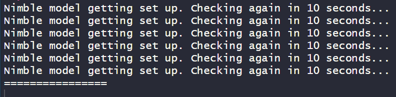
      cat(
        paste(
          "Nimble model getting set up. Checking again in",
          sleep_length * 2,"seconds...\n"
        )
      )
      Sys.sleep(sleep_length * 2)
      next
    } else {
      nran <- nchar(tmp[length(tmp)])
      setTxtProgressBar(pb, nran)
      Sys.sleep(sleep_length)
      
      if(substr(tmp[length(tmp)],nran,nran) == "|"){
        is_running <- FALSE
        cat("\n Model running complete!\n")
      }
    }
  }
}

As an example, I put together a script that fits a multi-species occupancy model and uses the function above(see this GitHub repository here). Note that the model fitting process has to be fully self-contained in it’s own script, as you need to send that to the console using a shell() call with the argument wait set to FALSE. Doing so let’s you continue running commands in R, which is what we need to do in order to call check_progress_mcmc().

The example.R script in that repo is the one you would run in your R session to try this out, though you do need the rest of the files on the repository for it to run correctly:

library(nimble)
library(doParallel)

# load the objects that need to be available to the cmd line
# and the R global environment. This includes
# --- 
# n_chains: number of chains to fit
# n_iterations: number of iterations for each model
# my_outfile: where the outfile text file should be located

source("./R/params.R")

# load the function to track progress. It opens up
#  the outfile, and looks for the progress bar that 
#  nimble creates in the file. 
source("./R/check_progress_mcmc.R")

# Delete the temporary file if it exists
if(
  file.exists(
    my_outfile
  )
){
  file.remove(my_outfile)
}

# Send the model to the command line which will fit it,
#  and save the output.
shell(
  "Rscript ./R/msom_mcmc.R",
  wait = FALSE
)
# just wait a little bit for the cluster to get spun up
Sys.sleep(2)
# and check your progress!
check_progress_mcmc(
  outfile = my_outfile,
  nchain = n_chains
)

# remove the outfile when done
file.remove(my_outfile)

# read in the model
model <- readRDS(
  "./mcmc_output/model_fit_2021-11-11.RDS"
)

And here is my little progress bar I get to see while my model is fitting in parallel!

It's a progress bar

And just in case you are interested, here is the code to set up and fit the model in NIMBLE (i.e., ./R/msom_mcmc.R).

# Read in the data
library(nimble)
library(doParallel)

source("./R/params.R")

 # start up the cluster
my_cluster <- makeCluster(
  n_chains,
  outfile = my_outfile
)

# site by species matrix, max number of surveys = 4
y <- read.csv("./data/species_data.R")

# design matrix
x <- read.csv("./data/design_matrix.R")

# query some values we'd need for the model
nsite <- nrow(y)
nspecies <- ncol(y)
nsurvey <- 4

# the data list for nimble
data_list <- list(
  y=y,
  design_matrix_psi = x,
  design_matrix_rho = x
)

# The constant list for nimble
constant_list <- list(
  # Number of sites
  nsite = nsite,
  # Number of repeat samples
  nsurvey = nsurvey,
  # number of species
  nspecies = nspecies,
  # design matrices for all models
  design_matrix_psi = x,
  design_matrix_rho = x,
  # number of parameters for each model
  npar_psi = ncol(x),
  npar_rho = ncol(x)
)

# the nimble model, written so that it can be run in parallel (i.e.,
#  the whole thing is written as one big function).
msom_mcmc <- function(seed, data_list, constant_list, niter = n_iterations){
  library(nimble)
  
  # The multi-species occupancy model
  msom_code <-nimble::nimbleCode(
    {
      for(site in 1:nsite){
        for(species in 1:nspecies){
          # logit linear predictor occupancy
          logit(psi[site,species]) <- inprod(
            beta_psi[species, 1:npar_psi],
            design_matrix_psi[site,1:npar_psi]
          )
          z[site,species] ~ dbern(
            psi[site,species]
          )
          # logit linear predictor detection
          logit(rho[site,species]) <- inprod(
            beta_rho[species,1:npar_rho],
            design_matrix_rho[site,1:npar_rho]
          )
          y[site,species] ~ dbin(
            rho[site,species] * z[site,species],
            nsurvey
          )
        }
      }
      # priors for occupancy
      for(psii in 1:npar_psi){
        beta_psi_mu[psii] ~ dlogis(0,1)
        tau_psi[psii] ~ dgamma(0.001,0.001)
        sd_psi[psii] <- 1 / sqrt(tau_psi[psii])
        for(species in 1:nspecies){
          beta_psi[species,psii] ~ dnorm(
            beta_psi_mu[psii],
            tau_psi[psii]
          )
        }
      }
      # priors for detection
      for(rhoi in 1:npar_rho){
        beta_rho_mu[rhoi] ~ dlogis(0,1)
        tau_rho[rhoi] ~ dgamma(0.001,0.001)
        sd_rho[rhoi] <- 1 / sqrt(tau_rho[rhoi])
        for(species in 1:nspecies){
          beta_rho[species,rhoi] ~ dnorm(
            beta_rho_mu[rhoi],
            tau_rho[rhoi]
          )
        }
      }
    }
  )
  
  # initial value function for the model
  my_inits <- function(){
    list(
      z = matrix(
        1,
        nrow = constant_list$nsite,
        ncol = constant_list$nspecies
      ),
      beta_psi = matrix(
        rnorm(constant_list$npar_psi * constant_list$nspecies),
        nrow  = constant_list$nspecies,
        ncol = constant_list$npar_psi),
      beta_rho = matrix(
        rnorm(constant_list$npar_psi * constant_list$nspecies),
        nrow  = constant_list$nspecies,
        ncol = constant_list$npar_psi)
    )
  }
  
  # set up the model
  msom <- nimble::nimbleModel(
    code = msom_code,
    name = "msom",
    constants = constant_list,
    data = data_list,
    inits = my_inits()
  )
  
  # you need to compile the model before
  # you modify the samplers.
  tmp_msom <- nimble::compileNimble(
    msom
  )
  # configure the model
  msom_configure <- nimble::configureMCMC(
    msom
  )
  # change the samplers
  msom_configure$addSampler(
    target = c("beta_psi_mu", "beta_psi"),
    type = "RW_block",
    control = list(adaptInterval = 100)
  )
  msom_configure$addSampler(
    target = c("beta_rho_mu", "beta_rho"),
    type = "RW_block",
    control = list(adaptInterval = 100)
  )
  # add monitors
  msom_configure$setMonitors(
    c(
      "beta_psi_mu", "beta_psi", "beta_rho_mu",
      "beta_rho", "sd_psi", "sd_rho"
    )
  )
  # going to sample the latent state as well,
  # but sample it less than the other parameters
  msom_configure$setMonitors2("z")
  msom_configure$setThin2(5)
  # build the model
  msom_build <- nimble::buildMCMC(
    msom_configure
  )
  # compile the model a second time,
  # reset functions because we added
  # different samplers.
  msom_compiled <- nimble::compileNimble(
    msom_build,
    project = msom,
    resetFunctions = TRUE
  )
  # fit the model
  results <- nimble::runMCMC(
    msom_compiled,
    niter = niter,
    setSeed = seed,
    inits = my_inits()
  )
  return(results)
}

# fit the model

chain_output <- parLapply(
  my_cluster,
  X = 1:n_chains,
  fun = msom_mcmc,
  data_list = data_list,
  constant_list = constant_list,
  niter = n_iterations
)
stopCluster(my_cluster)

saveRDS(
  chain_output,
  paste0(
    "./mcmc_output/model_fit_",Sys.Date(),".RDS"
  )
)

Written on November 11, 2021