Mason Fidino

When cleaning data for different analyses one of the first things you need to do is determine if there are any data entry errors present. For spatial coordinate data, this would mean plotting the points out on a map to determine if they fall within the expected region of interest. For example, if I am working with data in Chicago, Illinois, are the points in Chicago?

From my experience, spatial data is rife with errors. Some common errors I’ve experienced way too often include:

• Latitude and longitude have swapped places.
• The decimal is not in the correct location when working with lat / long data in decimal degrees.
• Latitude or longitude are listed as positive when they should actually be negative.
• If working with coordinates in universal transverse mercator (UTM), the UTM zone is not supplied, or is incorrect.

To plot out the points onto a map though, you need a map to plot on. If you are working with data in a region you’ve already got a raster or a shapefile of, it is easy enough to pull that in and plot on top of. However, what if you do not have a map available? Or what if you are working with data from all over the world and you don’t want to have to hunt down shapefiles for every study area?

Recently, I had these exact issues trying to validate spatial data while helping clean data for the Global Animal Diel Activity Project. Dr. Kadambari Devarajan and I tasked ourselves with getting the data ready for analysis, and I jumped at cleaning the spatial side of things up while Dr. Devarajan addressed date/time issues with camera trap images (of which there were many, as is typical for camera trapping projects).

For the spatial data, the best “check out the data” solution I found was to use the mapview package in R, which lets you spin up interactive maps from sf objects (among other classes). This was helpful if I just wanted to quickly look at data from one area, but with over 160 camera trapping projects in this analysis I needed to be able to automate image creation. But before we get to that, here is just a brief example of how to look at some spatial points from a single location. Note that while this first bit of code here will work with the version of mapview currently on CRAN, I suggest you download the version on GitHub as you will need it in order to correctly save images later. We’ll also load some other packages we’ll need to do some image manipulation later in this post.

# Note: I had to install mapview from github via:
remotes::install_github("r-spatial/mapview")

# for this to work. You need access to the webshot2() function
#  in order to get the points to be visible.

library(sf)
sf::sf_use_s2(FALSE)
library(mapview)
library(magick)

# You would likely read in your data instead, but this
#  is a little toy example.
my_sites <- data.frame(
  longitude = c(-87.707062, -87.607407, -87.652016,-87.652016),
  latitude = c(41.902840, 41.835289, 41.927826, 41.824289)
)

# convert to an sf object
my_sites <- sf::st_as_sf(
  my_sites,
  coords = c("longitude","latitude"),
  crs = 4326 # lat/long coordinate reference system
)

# just take a look at it using mapview
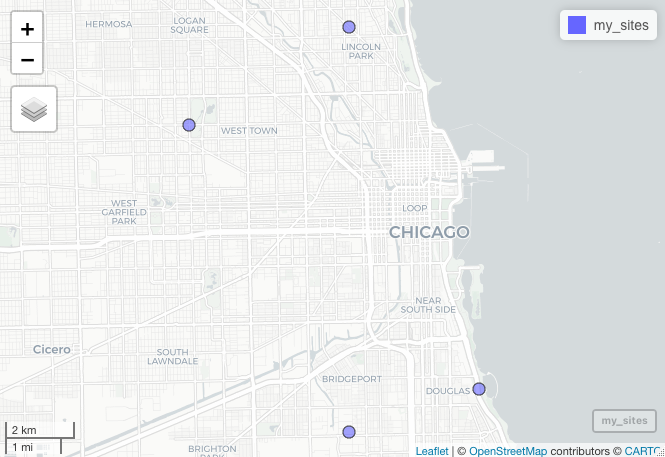
mapview::mapview(
  my_sites
)

The output from mapview automatically generates an interactive map that you can zoom into your points with, and would look something like this in R.

While checking the validity of the data for this project I did not want to have to interactively “assess” the coordiantes. It would take too much time, and I would not easily be able to send any problems I identified to collaborators. Thus, I needed to save static images instead of interactive maps. Likewise, to validate the spatial locations, we probably want to be able to see it at multiple scales to determine their validity. For example, having one zoomed out plot at the country scale to determine the points fall within the correct country and another more zoomed in plot around the sites. To do this with mapview, we need to make sure the phantomjs is installed as the webshot package (which mapview depends on) uses it to take a ‘snapshot’ of the html file spun up by mapview::mapview(). To do so in R, you can simply run:

if(!webshot::is_phantomjs_installed()){
  webshot::install_phantomjs()
}

Following this, we use the mapview::mapshot2() function to save a static image from mapview (which is why we needed to install mapview from GitHub). But first, it would probably help to make sure we are only plotting unique locations onto a map, as we don’t plot redundant points.

# step 1: Go from possibly repeat location data
#  down to a single point per location.
# get coordinate reference system
my_crs <- sf::st_crs(my_sites)
# and the spatial coordiantes of the sites
tmp <- sf::st_coordinates(my_sites)
# subset down to unique locations with x and y
tmp <- tmp[!duplicated(tmp),]
tmp <- tmp[complete.cases(tmp),]
tmp <- data.frame(tmp)
# give a site column
tmp$site <- 1:nrow(tmp)
# change back to an sf object
tmp <- sf::st_as_sf(
  tmp,
  coords = c("X","Y"),
  crs = my_crs
)

Now that we just have unique locations (in this toy example we already had unique locations, but that may not be the case with other datasets you encounter), we can create assign the output of mapview::mapview() as an object and feed it into mapview::mapshot2() to save our standard ‘zoomed in’ image.

map_close <- mapview::mapview(
  tmp,
  legend = FALSE
)

# do first plot
mapview::mapshot2(
  map_close,
  file = "tmp_close.png"
)

To zoom out a bit, we need to use the leaflet package to specify some options for the minimum and maximum zoom. I’ve found that a zoom of 3 is sufficient if you want to see where the points like within a given country.

# then do the second, further out this time
map_far <- mapview::mapview(
  tmp,
  legend = FALSE,
  map = leaflet::addTiles(
    leaflet::leaflet(
      options = leaflet::leafletOptions(minZoom = 3, maxZoom = 3)
    )
  )
)

# make a temporary file
mapview::mapshot2(
  map_far,
  file = "tmp_far.png"
)

At this point, we have two separate images, let’s combine them into a single file and delete these temporary images. This is easy enough to do with the magick package, which is a useful wrapper package that leverages the ImageMagick command line tool.

# concatenate both images into a single figure
widemap <- magick::image_append(
  c(
    magick::image_read(
      "tmp_far.png"
    ),
    magick::image_read(
      "tmp_close.png"
    )
  )
)
# and save it
magick::image_write(
  widemap,
  path = "my_chicago_sites.png"
)
# delete temporary images
file.remove("tmp_far.png")
file.remove("tmp_close.png")

And there you have it! Here is what these points would look like at two scales in Chicago.

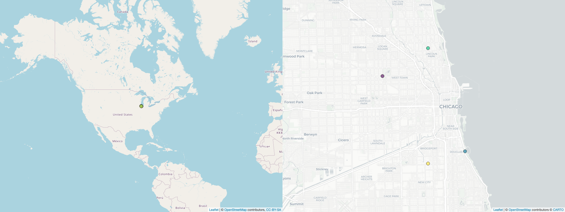
Finally. It is simple enough to wrap the code above into a function so that you can easily iterate through a set of study areas and plot out one set of maps for each study within a for loop. Here is the function I used for this (note that in this function if phantomjs is not installed on your local computer it will do it for you).

plot_map <- function(my_data, output){
  # my_data: an sf object of spatial points
  # output: a character object that specifies that saved png image (e.g. "./plots/chicago_sites.png")

  if(!"sf" %in% class(my_data)){
    stop("File must be sf class")
  }
    # step 1: Go from possibly repeat location data
    #  down to a single point per location.
    # get coordinate reference system
    my_crs <- sf::st_crs(my_data)
    # and the spatial coordiantes of the sites
    tmp <- sf::st_coordinates(my_data)
    # subset down to unique locations with x and y
    tmp <- tmp[!duplicated(tmp),]
    tmp <- tmp[complete.cases(tmp),]
    tmp <- data.frame(tmp)
    # give a site column
    tmp$site <- 1:nrow(tmp)
    # change back to an sf object
    tmp <- sf::st_as_sf(
      tmp,
      coords = c("X","Y"),
      crs = my_crs
    )
    # install webshot if you need to.
    if(!webshot::is_phantomjs_installed()){
      webshot::install_phantomjs()
    }
    # specif
    map_close <- mapview::mapview(
      tmp,
      legend = FALSE
    )
    # do first plot
    mapview::mapshot2(
      map_close,
      file = "tmp_close.png"
    )
    # then do the second, further out this time
    map_far <- mapview::mapview(
      tmp,
      legend = FALSE,
      map = leaflet::addTiles(
        leaflet::leaflet(
          options = leaflet::leafletOptions(minZoom = 3, maxZoom = 3)
        )
      )
    )
    # make a temporary file
    mapview::mapshot2(
      map_far,
      file = "tmp_far.png"
    )
    # concatenate both images into a single figure
    widemap <- magick::image_append(
      c(
        magick::image_read(
          "tmp_far.png"
        ),
        magick::image_read(
          "tmp_close.png"
        )
      )
    )
    # and save it
    magick::image_write(
      widemap,
      path = output
    )
    # delete temporary images
    file.remove("tmp_far.png")
    file.remove("tmp_close.png")
}

plot_map(
  my_sites,
  "chicago_sites.png"
)