How to interpret and make plots with a Bayesian implementation of the Rota et al. (2016) multi-species occupancy model for interacting species
In the past few years I have had the opportunity to either review a decent number of papers that have used the Rota et al. (2016) occupancy model or talk to graduate students that are interested in applying that model (or other offshoots of that model) to their own data. Based on this, I have found two issues that researchers commonly have. First, the model can be difficult to interpret (i.e., understanding what the model does and what the parameter estimates mean). Second, the model can be difficult to make predictions with. This second issue has gotten a bit easier now that the model has been rolled into the unmarked package. However that implementation won’t allow you to incorporate species interactions into the observational level of the model, which can be limiting (e.g., a prey species may be less detectable in the presence of a predator, but that cannot be estimated in unmarked::occuMulti()). As such, you may end up wanting to write your own model in nimble, JAGS, or stan, but unless you have access to the second volume of Applied Hierarchical Modeling in Ecology, there really are no good examples of how to take the MCMC outputs from this model and make some figures with it.
As such, in this post I’m going to cover how to interpret the parameters from this model in a statistical sense, and using some real camera trap data my colleagues and I at the Lincoln Park Zoo collected throughout Chicago, fit the model and make some figures of the results. Finally, at the end, I will provide my own ecological interpretation of the results from this model fit.
What I am not going to cover in this post is all the mathematical details of this model. Why? Because the Rota et al. (2016) paper is not paywalled, you can read it there! However, one thing I will note that is a deviation from the Rota et al. model is that I use a Categorical distribution instead of a multivariate Bernoulli distribution. Save for how you set up your response variables, they are equivalent distributions. However, the multivariate Bernoulli distribution is not a standard distribution in nimble, JAGS, or stan and so you’d have to write custom code for it. Conversely, the Categorical distribution is a standard distribution in those languages, so it is a much easier option to use. For example, when I generalized the Rota et al. (2016) model to a dynamic model, I used the Categorical distribution instead.
Links to different parts of this post
- The model and all those confusing parameters
- Estimating interactions between gray squirrel and coyote throughout Chicago
- Interpreting the model output
- Make some plots of the results
- On the difference between ecological and statistical interactions
I also link to it below, but just to make it more visible, all the data and code to recreate the analysis and plot the results can be found in this GitHub repo.
The model and all those confusing parameters
Honestly, I think the most confusing part with respect to this model is that some of the model parameters are used in multiple logit-linear predictors. Take, for example, the two species representation of the model. With two species, there are four possible states: 1) both species are not present, 2) species A is present, 3) species B is present, and 4) species A and B are present. Given \(N\) possible states, there are \(N-1\) linear predictors and that last state (species A and B) uses ALL of the parameters and covariates in state “species A is present” and “species B is present” PLUS more (if you add them to the model). For an intercept only model, the linear predictors of each state for the latent process is: \(\begin{eqnarray} \beta^{\psi_1} &=& \text{exp}(0) = 1 \\ \beta^{\psi_2} &=& \text{exp}(a_0) \\ \beta^{\psi_3} &=& \text{exp}(b_0) \\ \beta^{\psi_4} &=& \text{exp}(a_0 + b_0 + c_0) \end{eqnarray}\)
And to convert these back to a probability, you just use the softmax function (i.e., divide each linear predictor by the sum of all four linear predictors):
\[\begin{eqnarray} \psi_1 &=&\frac{\beta^{\psi_1}}{\beta^{\psi_1} + \beta^{\psi_2} + \beta^{\psi_3} + \beta^{\psi_4}} = \frac{1}{1 + \text{exp}(a_0) + \text{exp}(b_0) + \text{exp}(a_0 + b_0 + c_0)} \\ \psi_2 &=&\frac{\beta^{\psi_2}}{\beta^{\psi_1} + \beta^{\psi_2} + \beta^{\psi_3} + \beta^{\psi_4}} = \frac{\text{exp}(a_0)}{(1 + \text{exp}(a_0) + \text{exp}(b_0) + \text{exp}(a_0 + b_0 + c_0)} \\ \psi_3 &=&\frac{\beta^{\psi_3}}{\beta^{\psi_1} + \beta^{\psi_2} + \beta^{\psi_3} + \beta^{\psi_4}} = \frac{\text{exp}(b_0)}{(1 + \text{exp}(a_0) + \text{exp}(b_0) + \text{exp}(a_0 + b_0 + c_0)} \\ \psi_4 &=&\frac{\beta^{\psi_5}}{\beta^{\psi_1} + \beta^{\psi_2} + \beta^{\psi_3} + \beta^{\psi_4}} = \frac{\text{exp}(a_0 + b_0 + c_0)}{(1 + \text{exp}(a_0) + \text{exp}(b_0) + \text{exp}(a_0 + b_0 + c_0)} \end{eqnarray}\]In it’s intercept only form, a two species model like this would have three parameters in the latent state.
- \(a_0\): The log-odds of occupancy for species A given the absence of species B.
- \(b_0\): The log-odds of occupancy for species B given the absence of species A.
- \(c_0\): The log-odds difference in occupancy of both species occuring together.
That first two parameters, which Rota et al. (2016) call first-order parameters, are always going to be related to just one species. That last parameter, which is the tricky one, is called a second-order parameter because it is related to two species. To me, it helps to think of second order parameters as a statistical interaction term. A statistical interaction term means that two or more variables (i.e., \(a_0\) and \(b_0\)), may interact in a non-additive way. So, if \(c_0\) is positive, that means that both species occur together more than you would expect by chance and if \(c_0\) is negative that means that both species occur together less than you would expect by chance.
Breaking this down further, let’s say the probability of occupancy of species A is \(0.4\) and species B is \(0.7\). Just based off of random chance, we would expect these species to occur together in about half of the sites we would monitor (i.e., \(0.4 \times 0.7 = 0.49\)). Let’s say we go out and find that they occur together 90% of the time. If we fit this model to these data then we would expect \(c_0\) to be positive. Conversely, if we look at the data and see that they occur together 20% of the time then \(c_0\) would likely be negative. And, just to be complete, if we collected our data and saw that they occurred together 49% of the time, then \(c_0\) would likely get estimated to be zero (or something very close to that).
An incredible selling point of this model, however, is that you can also include spatial or temporal covariates on all of these linear predictors. Now, you do not need to include the same covariates in each linear predictor of this model, and sometimes you would have good reason not to (e.g., if you knew that your species are associated to different environmental features). But in this case we will just use the same generic covariate, \(x\), in each. For \(i\) in \(1, \cdots, I\) sites the logit linear predictors could be
\[\begin{eqnarray} \beta^{\psi_1}_i &=& 1 \\ \beta^{\psi_2}_i &=& \text{exp}(a_0 + a_1 \times x_i) \\ \beta^{\psi_3}_i &=& \text{exp}(b_0+ b_1 \times x_i) \\ \beta^{\psi_4}_i &=& \text{exp}(a_0 + a_1 \times x_i + b_0 + b_1 \times x_i + c_0 + c_1 \times x_i ) \end{eqnarray}\]Again, we see here that all of the parameters from state 2 & 3 are within the linear predictor of state 4. With the addition of a single covariate into each of these linear predictors we have added three more model parameters.
- \(a_1\): The log-odds change in occupancy for species A when species B is absent given a one unit increase in x.
- \(b_1\): The log-odds change in occupancy for species B when species A is absent given a one unit increase in x.
- \(c_1\): How the log-odds change in occupancy of species occurring together differs from their respective first-order slope terms given a one unit increase in x.
To understand this a little better, here is a small example in R where we can see how the probability of occupancy for each state changes with the inclusion and removal of slope terms, as well as second-order parameters. In all of these examples species A is more common than species B (i.e., has a more positive first-order intercept). I also introduce here the idea of marginal occupancy probabilities. These represent the probability of occupancy for a given species overall (i.e., irrespective of the presence of the other species) and are easy to calculate. For example, the marginal probability of occupancy for species A would be the summed occupancy probabilities for state 2 (i.e., species A present) and state 4 (i.e., species A & B present). On to the code.
# Example one: Species occur together as often as you would expect
#  by chance. No slope terms, second-order parameters set to 0.
a0 <- 1
b0 <- -0.5
c0 <- 0

# two, species, so four states
beta_psi <- rep(NA, 4)

# state 1: species not present
beta_psi[1] <- 1

# state 2: species A present
beta_psi[2] <- exp(a0)

# state 3: species B present
beta_psi[3] <- exp(b0)

# state 4: speecies A & B present
beta_psi[4] <- exp(a0 + b0 + c0)

# convert to probability
psi <- beta_psi / sum(beta_psi)

# see that they occur together as much as you would expect by chance

# calculate the marginal occupancy of species A,
#  which is the sum of all states that include species A
marginal_occ_a <- psi[2] + psi[4]

# calculate the marginal occupancy of species B,
#  which is the sum of all states that include species B
marginal_occ_b <- psi[3] + psi[4]

# the product of these two should be equivalent to psi[4]
c(
  "product of marginal occupancy" =  marginal_occ_a * marginal_occ_b,
  "Probability of state 4" = psi[4]
)
# they are the same!
# product of marginal occupancy
# 0.2760043
# Probability of state 4
# 0.2760043


# Example two: Species occur more together than you would expect
#  by chance. No slope terms but a positive second-order parameter.
a0 <- 1
b0 <- -0.5
c0 <- 1.5

# two, species, so four states
beta_psi <- rep(NA, 4)

# state 1: species not present
beta_psi[1] <- 1

# state 2: species A present
beta_psi[2] <- exp(a0)

# state 3: species B present
beta_psi[3] <- exp(b0)

# state 4: speecies A & B present
beta_psi[4] <- exp(a0 + b0 + c0)

# convert to probability
psi <- beta_psi / sum(beta_psi)

# calculate the marginal occupancy of species A,
#  which is the sum of all states that include species A
marginal_occ_a <- psi[2] + psi[4]

# calculate the marginal occupancy of species B,
#  which is the sum of all states that include species B
marginal_occ_b <- psi[3] + psi[4]

# psi[4] should be greater than the product of the marginals
c(
  "product of marginal occupancy" =  marginal_occ_a * marginal_occ_b,
  "Probability of state 4" = psi[4]
)
# State 4 happens more than you would expect by chance
#  product of marginal occupancy
#  0.5889609
#  Probability of state 4
#  0.6307955

# However, look and see how common each community state is. They
#  occur together way more than they do alone!
round(psi,2)
# [1] 0.09 0.23 0.05 0.63

# Example three: Species occur more together than you would expect
#  by chance, but that decreases along an environmental gradient.
a0 <- 1
a1 <- 0.7
b0 <- -0.5
b1 <- 1.2
c0 <- 1.5
c1 <- -2

# choose three covariate values for sake of example
x <- c(-1,0,1)

# two, species, so four states, but with
#  three covariate values we need a matrix now.
beta_psi <- matrix(
  NA,
  ncol =4,
  nrow = length(x)
)

# fill in beta_psi with a loop
for(i in 1:nrow(beta_psi)){
  # state 1: species not present
  beta_psi[i,1] <- 1

  # state 2: species A present
  beta_psi[i,2] <- exp(a0 + a1 * x[i])

  # state 3: species B present
  beta_psi[i,3] <- exp(b0 + b1 * x[i])

  # state 4: speecies A & B present
  beta_psi[i,4] <- exp(a0 + a1 * x[i] + b0 + b1 * x[i] + c0 + c1 * x[i])
}


# convert to probability
psi <- sweep(
  beta_psi,
  1,
  rowSums(beta_psi),
  FUN = "/"
)

colnames(psi) <- c("none", "A", "B", "AB")

# look at probability of each state, we see that Pr(AB) goes down
#  as our environmental gradient increases (i.e., goes from
#  negative to positive).
round(psi,2)
#       none    A    B   AB
#  [1,] 0.09 0.13 0.02 0.76 # at x = -1
#  [2,] 0.09 0.23 0.05 0.63 # at x =  0
#  [3,] 0.07 0.36 0.13 0.44 # at x =  1
Okay, we’ve broken down the latent state of the model, let’s move to the observational process. Now this part of the model is honestly more confusing because there are 1) a lot of detection probabilities to calculate and 2) a bunch of different parameterizations you could use depending on what you are interested in estimating.
The unmarked::occuMulti() parameterization is the simplest as it assumes that the presence of one species does not
have an influence on the probability of detection of another species. Let \(\rho_A\) be the probability of detecting species A and \(\rho_B\) be the probability of detecting species B. We could then specify a square detection probability matrix, where the rows represent the true latent state and the columns represent the observed state, and as such the row sums must equal 1.
Note the zeroes in the matrix here. This means that given the true state (i.e., what row you are on), you cannot observe this state. For example, if you are in state “no species present” then you cannot detect species A, B, or both together. In this case here if you wanted to add covariates to this level of the model you would 1) add a site and possibly observation level index to your detection matrix, and 2) use the logit link. If we just had some site-specific variation in detection probability that could look like
\[\begin{eqnarray} \text{logit}(\rho_{Ai}) &=& f_0 + f_1 \times x_i \\ \text{logit}(\rho_{Bi}) &=& g_0 + g_1 \times x_i \end{eqnarray}\]However, if you want to start adding interactions among species in this level of the model, then we have to return back to using the softmax function instead of the logit link. Let’s say that you want to determine if detecting both species is not just \(\rho_A \times \rho_B\). Just like with the latent state model we can just add a second order parameter to a log-odds detection matrix. Assuming an intercept only model that would be.
\[\begin{eqnarray} \beta^{\rho_1} &=& \text{exp}(0) = 1 \\ \beta^{\rho_2} &=& \text{exp}(f_0) \\ \beta^{\rho_3} &=& \text{exp}(g_0) \\ \beta^{\rho_4} &=& \text{exp}(f_0 + g_0 + h_0) \end{eqnarray}\]And then we drop these linear predictors into a matrix \(\boldsymbol{\omega}\)
\[\boldsymbol{\omega} = \begin{bmatrix} 1 & 0 & 0 & 0 \\ 1 & \beta^{\rho_2} & 0 & 0 \\ 1 & 0 & \beta^{\rho_3} & 0 \\ 1 & \beta^{\rho_2} & \beta^{\rho_3} & \beta^{\rho_4} \end{bmatrix}\]To convert this matrix back to a probability you would just apply the softmax function to each row (i.e., take the sum of each row, and divide each element of that row by the sum). Note here that this parameterization only ‘turns on’ the second-order parameter \(h_0\) when we are in state 4.
Finally, maybe you would be interested in seeing if the detection probability of each species varies given the presence of the other. For the observation level of the model you can actually create directional interactions so you could estimate how the probability of detecting one species may vary given the presence of the other. For this, we need to specify a few more linear predictors that get used once again in the final row of \(\boldsymbol{\omega}\). Also note I’m changing my notation a bit, so instead of states 1 through 4 I have explicit references to what each linear predictor represents (U = unoccupied).
\[\begin{eqnarray} \beta^{\rho_U} &=& \text{exp}(0) = 1 \\ \beta^{\rho_A} &=& \text{exp}(f_0) \\ \beta^{\rho_B} &=& \text{exp}(g_0) \\ \beta^{\rho_{A|B}} &=& \text{exp}(f_0 + h_0) \\ \beta^{\rho_{B|A}} &=& \text{exp}(g_0 + j_0) \\ \beta^{\rho_{AB}} &=& \text{exp}(f_0 + h_0 + g_0 + j_0) \end{eqnarray}\]Here, \(f_0\) and \(g_0\) are the first-order detection parameters while \(h_0\) and \(j_0\) are the second-order detection parameters. More specifically, \(h_0\) is the log-odds difference in detecting species A when species B is present whereas \(j_0\) is the log-odds difference in detecting species B when species A is present.
And then we drop these linear predictors into \(\boldsymbol{\omega}\)
\[\boldsymbol{\omega} = \begin{bmatrix} 1 & 0 & 0 & 0 \\ 1 & \beta^{\rho_A} & 0 & 0 \\ 1 & 0 & \beta^{\rho_B} & 0 \\ 1 & \beta^{\rho_{A|B}} & \beta^{\rho_{B|A}} & \beta^{\rho_{AB}} \end{bmatrix}\]Estimating interactions between gray squirrel and coyote throughout Chicago
My colleagues and I at the Lincoln Park Zoo have been doing camera trapping in urban green space along a gradient of urban intensity throughout Chicago, Illinois for over a decade. To be honest, the reason why I got interested in statistics was because of this dataset. There were so many questions we were interested in answering with these data and, at the time, there were not models that were available to answer them with! For this example, I am just going to grab one season’s worth of data for coyote (Canis latrans) and eastern gray squirrel (Sciurus carolinensis) at 92 sites throughout the Chicago metropolitan area. The data have already been assembled into daily detection histories for each species. However, because we are using the Categorical distribution in our model, we need to go from the seperate binary detection / non-detection states for each species and convert them to observational states. Likewise, we are going to add an urban intensity covariate to this model, which I constructed by applying Principal Component Analysis (PCA) to the proportion of impervious cover within 1 km of each site, the mean Normalized Difference Vegetation Index (NDVI) within 1 km of each site, and the human population density within 1 km of each site. I used PCA here because urbanization often influences multiple environmental features in tandem. So in Chicago, for example, these three variables are often incredibly correlated to one another. So, in my opinion, it’s better to capture the gradient via PCA instead of just choosing one of these highly correlated variables to include. All data and code for this can be found on this GitHub repo, but the code to fit the model in nimble is here. In fact, you won’t be able to run this code here without going to that repo because you won’t have the data otherwise!
For this model I chose the second detection level parameterization for simplicity (i.e., the probability of detecting the species together given both present may be different). However, because coyotes can eat squirrels, it would probably make more sense to set up your model so that gray squirrel detections could vary given the presence of coyote whereas coyote detections are independent of gray squirrel.
library(nimble)
library(dplyr)
library(stringi)
library(MCMCvis)

# Read in the data
data <- read.csv(
  "./data/squirrel_coyote.csv"
)

# take a little look at the organization of the data
dplyr::glimpse(data)

# Rows: 184
# Columns: 40
# $ Species <chr> "coyote", "coyote", "coy…
# $ Site    <chr> "D02-BMT1", "D02-HUP0", …
# $ Day_1   <int> NA, NA, NA, NA, NA, NA, …
# $ Day_2   <int> NA, 0, NA, 0, NA, 0, 0, …
# $ Day_3   <int> 0, 0, NA, 0, NA, 0, 0, 0…
# $ Day_4   <int> 0, 0, NA, 0, NA, 0, 0, 0…
# $ Day_5   <int> 0, 0, NA, 0, NA, 0, 0, 0…

# figure out some general info about the data
nsite <- length(
  unique(
    data$Site
  )
)

ndays <- length(
  grep(
    "Day",
    colnames(
      data
    )
  )
)

# Determine community state at for each
#  secondary sampling period.

# This will store all of our detection
#  non-detection data
com_state <- matrix(
  NA,
  ncol = ndays,
  nrow = nsite
)

# paste the species data together. The data has been
#  sorted by site and species already (alphabetically),
#  so it would go coyote data, then gray squirrel
#  data.
sp_combo <- data %>%
  dplyr::group_by(Site) %>%
  dplyr::summarise_at(
    dplyr::vars(
      dplyr::starts_with("Day")
    ),
    .funs = function(x) paste0(x, collapse = "-")
  )

# construct a map for what each combo means
combo_map <- data.frame(
  # what we have
  combo = c("NA-NA", "0-0", "1-0", "0-1", "1-1"),
  # what the model wants
  value = c(NA, 1,2,3,4),
  # to remember what each one means
  meaning = c(
    "no sampling",
    "no species",
    "coyote",
    "gray squirrel",
    "coyote & gray squirrel"
  )
)

# use the combo_map and sp_combo to construct the
#  detection matrix. Easiest way to do this is
#  with this stringi function for each column.
for(i in 1:ncol(com_state)){
  day_vec <- sp_combo[,paste0("Day_",i), drop = TRUE]
  day_vec <- stringi::stri_replace_all_fixed(
    day_vec,
    combo_map$combo,
    combo_map$value,
    vectorize_all = FALSE
  )
  # put into the detection matrix
  com_state[,i] <- as.numeric(day_vec)
}

# com_state is what is the data we will supply to the model,
#  so let's pull in our covariate data.
covs <- read.csv(
  "./data/site_covariates.csv"
)

# scale the covariates
cov_scale <- covs %>%
  dplyr::summarise_if(
    is.numeric,
    scale
  )

# apply PCA to generate an urbanization score
(cov_pca <- prcomp(
  cov_scale
))

#                           PC1        PC2         PC3
# Impervious         -0.6360670  0.3094596 0.706861714
# Ndvi                0.6363000 -0.3078588 0.707350923
# Population_density -0.4365101 -0.8996987 0.001090312

# currently,these data represent a gradient of built environment when
#  negative to more vegetation when positive. Let's flip it so that
#  positive means more built environment. This is simple, just
#  multiply the loadings (rotation) and the first principal
#  component (x) by -1. Now, positive values are more urban
#  while negative values are more 'green.'

cov_pca$rotation[,1] <- cov_pca$rotation[,1] * -1
cov_pca$x[,1] <- cov_pca$x[,1] * -1


# put together lists for analysis
data_list <- list(
  # detection /non-detection data
  y = com_state,
  # design matrix for occupancy and detection,
  #  currently assuming the same covariates
  x = cbind(1, cov_pca$x[,1])
)

constant_list <- list(
  nsite = nsite,
  nvisit = ncol(com_state),
  nstate = dplyr::n_distinct(data$Species)^2,
  npar_psi = ncol(data_list$x),
  npar_rho = ncol(data_list$x)
)


# initial values function
inits <- function(){
  with(
    constant_list,
    {
      list(
        spA_psi = rnorm(npar_psi),
        spB_psi = rnorm(npar_psi),
        spAB_psi = rnorm(npar_psi),
        spA_rho = rnorm(npar_rho),
        spB_rho = rnorm(npar_rho),
        spAB_rho = rnorm(npar_rho),
        z = rep(nstate, nsite)
      )
    }
  )
}

# load the model
source("./nimble/rota_model.R")

my_model <- nimble::nimbleMCMC(
  code = rota_model,
  constants = constant_list,
  data = data_list,
  monitors = c(
    "spA_psi",
    "spB_psi",
    "spAB_psi",
    "spA_rho",
    "spB_rho",
    "spAB_rho"
  ),
  niter = 70000,
  nburnin = 20000,
  nchains = 2,
  thin = 2,
  inits = inits
)

# save the model output
saveRDS(
  my_model,
  "./nimble/mcmc_output.rds"
)
And before we get into the model summary, here is the nimble code for the model itself.
rota_model <- nimble::nimbleCode(
  {
    # latent state linear predictors
    # linear predictors. TS = True state
    # TS = U
    # The latent-state model
    for(site in 1:nsite){
      psi[site,1] <- 1
      # TS = A
      psi[site,2] <- exp(
        inprod(
          x[site,1:npar_psi],
          spA_psi[1:npar_psi]
        )
      )
      # TS = B
      psi[site,3] <- exp(
        inprod(
          x[site,1:npar_psi],
          spB_psi[1:npar_psi]
        )
      )
      # TS = AB
      psi[site,4] <- exp(
        inprod(
          x[site,1:npar_psi],
          spA_psi[1:npar_psi]
        ) +
        inprod(
          x[site,1:npar_psi],
          spB_psi[1:npar_psi]
        ) +
        inprod(
          x[site,1:npar_psi],
          spAB_psi[1:npar_psi]
        )
      )
      z[site] ~ dcat(
        psi[site,1:nstate]
      )
    }
    # The observation model linear predictors.
    # OS = Observed state
    for(site in 1:nsite){
      # OS = U
      rho[site,1] <- 1
      # OS = A
      rho[site,2] <- exp(
        inprod(
          x[site,1:npar_rho],
          spA_rho[1:npar_rho]
        )
      )
      # OS = B
      rho[site,3] <- exp(
        inprod(
          x[site,1:npar_rho],
          spB_rho[1:npar_rho]
        )
      )
      # OS = AB
      rho[site,4] <- exp(
        inprod(
          x[site,1:npar_rho],
          spA_rho[1:npar_rho]
        ) +
        inprod(
          x[site,1:npar_rho],
          spB_rho[1:npar_rho]
        ) +
        inprod(
          x[site,1:npar_rho],
          spAB_rho[1:npar_rho]
        )
      )
    }
    # And use these to fill in the rho detection matrix (rdm)
    # TS = U
    rdm[1:nsite,1,1] <- rho[1:nsite,1] # ------- OS = U
    rdm[1:nsite,1,2] <- rep(0, nsite) # -------- OS = A
    rdm[1:nsite,1,3] <- rep(0, nsite) # -------- OS = B
    rdm[1:nsite,1,4] <- rep(0, nsite) # -------- OS = AB
    # TS = A
    rdm[1:nsite,2,1] <- rho[1:nsite,1] # ------- OS= U
    rdm[1:nsite,2,2] <- rho[1:nsite,2] # ------- OS = A
    rdm[1:nsite,2,3] <- rep(0, nsite) # -------- OS = B
    rdm[1:nsite,2,4] <- rep(0,nsite) # --------- OS = AB
    # TS = B
    rdm[1:nsite,3,1] <- rho[1:nsite,1] # ------- OS = U
    rdm[1:nsite,3,2] <- rep(0, nsite) # -------- OS = A
    rdm[1:nsite,3,3] <- rho[1:nsite,3] # ------- OS = B
    rdm[1:nsite,3,4] <- rep(0, nsite) # -------- OS = AB
    # TS = AB
    rdm[1:nsite,4,1] <- rho[1:nsite,1] # ------- OS = U
    rdm[1:nsite,4,2] <- rho[1:nsite,2] # ------- OS = A
    rdm[1:nsite,4,3] <- rho[1:nsite,3] # ------- OS = B
    rdm[1:nsite,4,4] <- rho[1:nsite,4] # ------- OS = AB
    # observational model. z indexes the correct
    #   part of rdm
    for(site in 1:nsite){
      for(visit in 1:nvisit){
        y[site,visit] ~ dcat(
          rdm[
            site,
            z[site],
            1:nstate
          ]
        )
      }
    }
    # priors
    for(psii in 1:npar_psi){
      spA_psi[psii] ~ dlogis(0,1)
      spB_psi[psii] ~ dlogis(0,1)
      spAB_psi[psii] ~ dlogis(0,1)
    }
    for(rhoi in 1:npar_rho){
      spA_rho[rhoi] ~ dlogis(0,1)
      spB_rho[rhoi] ~ dlogis(0,1)
      spAB_rho[rhoi] ~ dlogis(0,1)
    }
  }
)
Interpreting the model output
Now, let’s take a look at the model summary, where species A = coyote and species B = gray squirrel. The parameter names should be pretty self explanatory, but just in case they are not to you here are some details. All second-order parameters have AB in them, whereas first-order parameters just have A or B respectively. Occupancy parameters are labeled psi and detection parameters are labeled rho. Finally, Intercepts all have [1] after them while the urban intensity slope terms have [2] after them.
# summarize model parameters
my_summary <- MCMCvis::MCMCsummary(
  my_model,
  digits = 2
)

#              mean    sd   2.5%   50%   97.5% Rhat n.eff
# spAB_psi[1] -0.19 0.630 -1.400 -0.20  1.1000    1  1402
# spAB_psi[2]  0.95 0.490  0.058  0.92  2.0000    1  1166
# spAB_rho[1]  0.36 0.250 -0.140  0.37  0.8200    1  4533
# spAB_rho[2] -0.37 0.190 -0.760 -0.36  0.0055    1  4743
# spA_psi[1]   0.57 0.560 -0.460  0.55  1.8000    1  1585
# spA_psi[2]  -0.70 0.380 -1.400 -0.71  0.0980    1  1770
# spA_rho[1]  -2.60 0.160 -2.900 -2.50 -2.2000    1  2628
# spA_rho[2]  -0.37 0.120 -0.610 -0.37 -0.1300    1  2622
# spB_psi[1]   1.20 0.490  0.250  1.20  2.2000    1  1667
# spB_psi[2]  -0.84 0.360 -1.600 -0.81 -0.2100    1  1285
# spB_rho[1]  -0.91 0.052 -1.000 -0.91 -0.8000    1 14993
# spB_rho[2]   0.26 0.035  0.190  0.26  0.3300    1 14632
Aside from the fact that it looks like I should sample this model a little longer to increase the effective sample size of the posteriors, here is what I see for the latent state of the model as a ‘first pass interpretation’.
- On average, gray squirrel are much more common than coyote (
spB_psi[1] > spA_psi[1]). - Both species are more common at lower levels of urban intensity (
spA_psi[2]andspB_psi[2]are negative). However, we have much stronger evidence of this relationship with gray squirrel because the 95% CI for spB_psi[2] does not bound zero (while spA_psi[2] does). - At an average location, there was insufficient evidence to determine that coyote and gray squirrel co-occur more or less than expected by chance (
spAB_psi[1]is close to zero and 95% CI bounds zero). - However, as urban intensity increases we have strong evidence that coyote and gray squirrel co-occur more than expected (
spAB_psi[2]is positive and 95% CI does not bound zero).
For the observational process we can see that:
- On average, daily detection probabilities are low for both species, but it is much lower for coyote (
spA_rho[1]andspB_rho[1]are negative, with the former being very negative). - Coyote detection probability decreases with urban intensity (
spA_rho[2]is negative and 95% CI does not bound zero) while gray squirrel detection probability increases with urban intensity (spB_rho[2]is positive and 95% CI does not bound zero). - We have insufficient evidence to determine if detecting coyote and gray squirrel on the same day given they both are present occurs more or less then we would expect relative to their baseline detection probabilities (
spAB_rho[1]trends positive but 95% CI bounds zero). - However, it seems as if a site is in ‘coyote & gray squirrel present’ we appear to be less likely to observe that state as urban intensity increases (
spAB_rho[2]is negative and BARELY bounds zero, it’s like a 94% probability of effect which is good enough for me to bet on).
Again, if this was for something beyond an example I would most certainly run this model more to increase the effective sample size. We want to ensure we have accurate 95% CI and with only about 1000 samples for these parameters I would want to boost that a bit. Conversely, instead of running the model for longer I could use slice samplers instead of the default Metropolis-Hasting algorithm that likely got used. Slice samplers are a bit slower but they often have a greater acceptance rate for proposals, which could in turn increase the effective sample size in the posterior.
Make some plots of the results
Anyways, let’s get on to plotting out the results here. To do so, we need to do a few things:
- Get the MCMC samples together in a usable format.
- Generate a design matrix for predictions.
- Make predictions for each state on the log-odds scale.
- Convert log-odds estimates to probabilities via the softmax function.
- Calculate median estimate and 95% CI of each probability.
It’s really easy to get the MCMC samples out of nimble. However, it puts them all in the same matrix which makes things difficult to work with. I created a utility function, split_mcmc(), which takes the output from nimble or JAGS and makes a named list with one element for each parameter type. The resulting output makes it look much more like what we coded up in nimble, which is going to make it way easier to make predictions with. But first, here is what the figure will look like when we are not. Not quite publication quality, but it’s a great start.
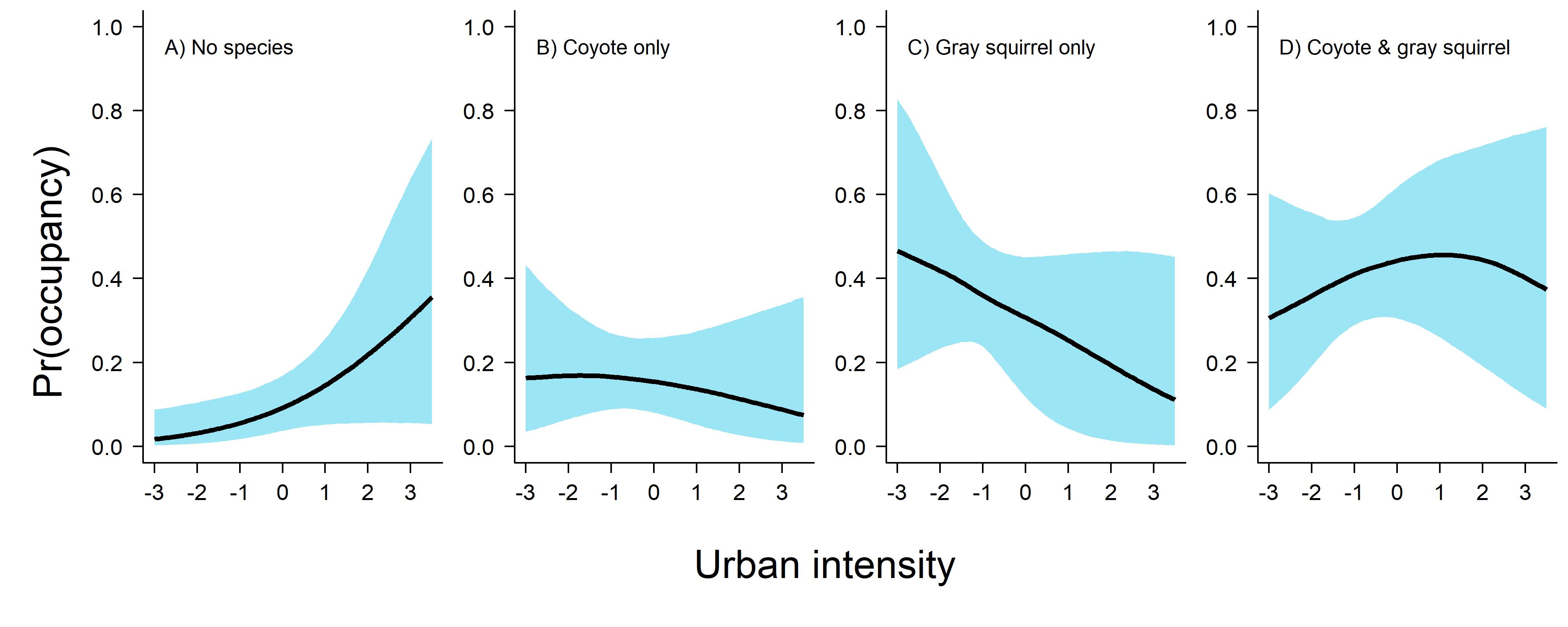
Before I share the code here, it’s important to note that while coyote & squirrel co-occurred more together as urbanization increased, it actually drops off a bit in favor of the state “no species present.” This is because the marginal occupancy of both of these species decreases with urban intensity and so the probability of detecting coyote only, gray squirrel only, or both species together lessens.
And here is the code to create the occupancy figure, which is the file "./R/plot_results.R" in this repo.
library(nimble)
library(MCMCvis)


# source split_mcmc(), which splits the mcmc output into useable pieces
source("./R/mcmc_utility.R")

# load in the model output
my_model <- readRDS(
  "./nimble/mcmc_output.rds"
)

# turn my_model into an MCMC matrix
mc <- do.call(
  "rbind",
  my_model
)

# sub-sample the mcmc matrix a bit as we don't really
#  need to make predictions with all 50K mcmc samples.
set.seed(554)
mc <- mc[
  sample(
    1:nrow(mc),
    10000
  ),
]

# and use split_mcmc()
mc <- split_mcmc(
  mc
)

# check out dimensions of one of the list elements.
#  for this example, each of them should have a number
#  of rows equal to the number of MCMC samples and a number
#  of columns equal to the number of parameters of that type.
dim(mc$spAB_psi)
#[1] 10000     2

# Recreate our PCA really quick so we know what range we
#  want to make predictions with. Again, we need to
#  multiply the principal component by -1 as we did
#  in fit_real_data.R (so positive values = more urban)


covs <- read.csv(
  "./data/site_covariates.csv"
)

# scale the covariates
cov_scale <- covs %>%
  dplyr::summarise_if(
    is.numeric,
    scale
  )

# apply PCA to generate an urbanization score
(cov_pca <- prcomp(
  cov_scale
))

cov_pca$rotation[,1] <- cov_pca$rotation[,1] * -1
cov_pca$x[,1] <- cov_pca$x[,1] * -1

# look at range of cov_pca$x[,1]
range(cov_pca$x[,1])

# [1] -3.010259  3.785600

# I need to choose some 'pretty' numbers based on that,
#  so we will go from -3 to 3.5. Adding a column of 1's
#  for the intercept

pred_mat <- rbind(
  1,
  seq(-3, 3.5, length.out = 200)
)

# generate predictions for each state. Put in an
#  array that is mcmc samples by ncol(pred_mat) by number of states.
beta_psi <- array(
  NA,
  dim = c(
    nrow(mc$spAB_psi),
    ncol(pred_mat),
    4
  )
)

# fill it in. No species is easy, it's just a 1.
beta_psi[,,1] <- 1

# Species A
beta_psi[,,2] <- exp(
  mc$spA_psi %*% pred_mat
)

# species B
beta_psi[,,3] <- exp(
  mc$spB_psi %*% pred_mat
)

# species A and B
beta_psi[,,4] <- exp(
  mc$spA_psi %*% pred_mat +
  mc$spB_psi %*% pred_mat +
  mc$spAB_psi %*% pred_mat
)

# convert to probability
psi <- array(
  NA,
  dim = dim(beta_psi)
)
pb <- txtProgressBar(max = ncol(pred_mat))
for(i in 1:ncol(pred_mat)){
  setTxtProgressBar(pb, i)
  psi[,i,] <- sweep(
    beta_psi[,i,],
    1,
    rowSums(beta_psi[,i,]),
    FUN = "/"
  )
}

# calculate median and quantiles with apply.
#  we choose 2 and 3 as margins as we want
#  to calculate these from the 10K mcmc samples
#  i.e., the first dimension.
psi_summary <- apply(
  psi,
  c(2,3),
  quantile,
  probs = c(0.025,0.5,0.975)
)

# get environmental covariate.
urb <- pred_mat[2,]

# make labels
my_labels <- c(
  "A) No species",
  "B) Coyote only",
  "C) Gray squirrel only",
  "D) Coyote & gray squirrel"
)

jpeg(
  "./plots/coyote_squirrel_occupancy.jpeg",
  width = 10,
  height = 4,
  units = "in",
  res = 400
)
layout(matrix(1:4, ncol = 4))
par(mar = c(4,3,0.5,0.5), oma = c(4,4,0,0), lend = 1)

# plot them out with a loop
for(i in 1:4){

  plot(
    1~1,
    type = "n",
    xlim = range(urb),
    ylim = c(0,1),
    bty = "l",
    xlab = "",
    ylab = "",
    las = 1,
    cex.axis = 1.3
  )
  # if first plot add axis titles
  if(i == 1){
    # add margin text in outer margin for y axis
    mtext(
      text = "Pr(occupancy)",
      side = 2,
      outer = TRUE,
      at = 0.5,
      line = 0.8,
      cex = 1.5
    )
    # add margin text in outer margin for x axis
    mtext(
      text = "Urban intensity",
      side = 1,
      outer = TRUE,
      at = 0.5,
      line = 0.8,
      cex = 1.5
    )
  }
  # add 95% CI
  polygon(
    x = c(
      urb,
      rev(urb)
    ),
    y = c(
      psi_summary[1,,i],
      rev(psi_summary[3,,i])
    ),
    col = "#9CE5F4",
    border = NA
  )
  # and median line
  lines(
    x = urb,
    y = psi_summary[2,,i],
    lwd = 3
  )
  text(
    x = -3,
    y = 0.95,
    labels = my_labels[i],
    pos = 4,
    cex = 1.2
  )
}
dev.off()
# script continues in next code chunk...
Doing the detection plots is a bit more involved because you would need to generate separate plots for each state. As this post is already getting long I”m just going to plot out the probability of detecting these species when they are in state 4 (i.e., they are together).
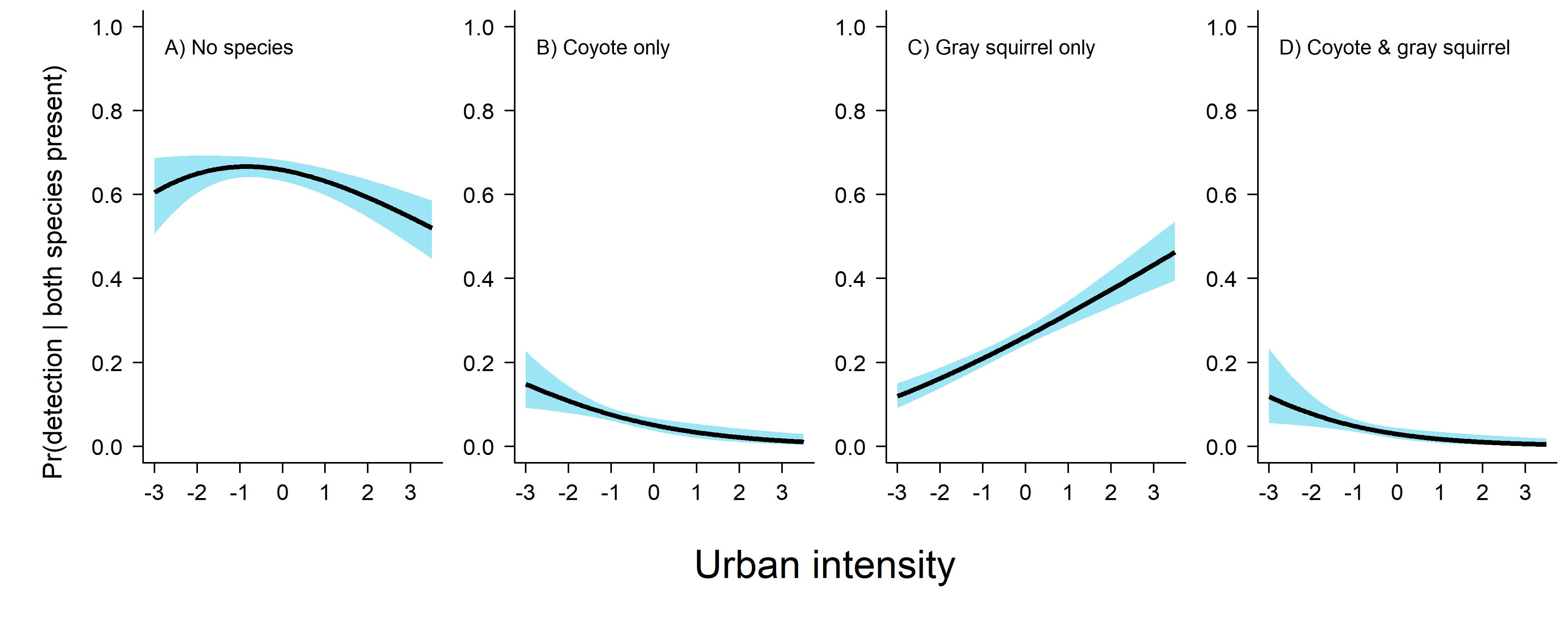
Looking at this figure here we can see that detecting gray squirrel on their own is the most likely thing to happen when both species are present, and we very seldomly detect the species on the same day. Here is the code I used to produce this plot.
# This is just a continuation of the "./R/plot_results.R" script...
beta_rho <- array(
  NA,
  dim = c(
    nrow(mc$spAB_rho),
    ncol(pred_mat),
    4
  )
)

# fill it in. No species is easy, it's just a 1.
beta_rho[,,1] <- 1

# Species A
beta_rho[,,2] <- exp(
  mc$spA_rho %*% pred_mat
)

# species B
beta_rho[,,3] <- exp(
  mc$spB_rho %*% pred_mat
)

# species A and B
beta_rho[,,4] <- exp(
  mc$spA_rho %*% pred_mat +
    mc$spB_rho %*% pred_mat +
    mc$spAB_rho %*% pred_mat
)

# convert to probability
rho <- array(
  NA,
  dim = dim(beta_rho)
)
pb <- txtProgressBar(max = ncol(pred_mat))
for(i in 1:ncol(pred_mat)){
  setTxtProgressBar(pb, i)
  rho[,i,] <- sweep(
    beta_rho[,i,],
    1,
    rowSums(beta_rho[,i,]),
    FUN = "/"
  )
}


# calculate median and quantiles with apply.
#  we choose 2 and 3 as margins as we want
#  to calculate these from the 10K mcmc samples
#  i.e., the first dimension.
rho_summary <- apply(
  rho,
  c(2,3),
  quantile,
  probs = c(0.025,0.5,0.975)
)

# and we can just barely modify the occupancy plot for plotting
#  this out now.

jpeg(
  "./plots/coyote_squirrel_detection.jpeg",
  width = 10,
  height = 4,
  units = "in",
  res = 400
)
layout(matrix(1:4, ncol = 4))
par(mar = c(4,3,0.5,0.5), oma = c(4,4,0,0), lend = 1)

# plot them out with a loop
for(i in 1:4){

  plot(
    1~1,
    type = "n",
    xlim = range(urb),
    ylim = c(0,1),
    bty = "l",
    xlab = "",
    ylab = "",
    las = 1,
    cex.axis = 1.3
  )
  # if first plot add axis titles
  if(i == 1){
    # add margin text in outer margin for y axis
    mtext(
      text = "Pr(detection | both species present)",
      side = 2,
      outer = TRUE,
      at = 0.5,
      line = 0.8,
      cex = 1
    )
    # add margin text in outer margin for x axis
    mtext(
      text = "Urban intensity",
      side = 1,
      outer = TRUE,
      at = 0.5,
      line = 0.8,
      cex = 1.5
    )
  }
  # add 95% CI
  polygon(
    x = c(
      urb,
      rev(urb)
    ),
    y = c(
      rho_summary[1,,i],
      rev(rho_summary[3,,i])
    ),
    col = "#9CE5F4",
    border = NA
  )
  # and median line
  lines(
    x = urb,
    y = rho_summary[2,,i],
    lwd = 3
  )
  text(
    x = -3,
    y = 0.95,
    labels = my_labels[i],
    pos = 4,
    cex = 1.2
  )
}
dev.off()
On the difference between ecological and statistical interactions
In closing, I just want to return back to one really important thing you must be cautious about when interpreting the results from these models: statistical interactions are not the same thing as ecological interactions. In the coyote & gray squirrel example, we estimated that they occurred together more often as urban intensity increased. This does not mean that these species have a mutualistic relationship. Likewise, if we estimated negative covariance among species that does not mean that these species are competing with one another, or one is inherently trying to avoid the other. More often then not with any of these community models that estimate interactions among species, it just means that there is some environmental gradient you did not include into the model that the two species positively or negatively covary along. When that gradient is not included, the covariance among species can binned into the interaction terms, which could result in strong ‘statistical interactions’ that actually have no ecological meaning.
As such, please be cautious when interpreting this class of models! My own cautious interpretation of the example above is that urbanization makes for strange bedfellows. In downtown Chicago, this means that species likely occupy the same habitat patch more often simply because that is what is available. Essentially, habitat is limited, and so the species are more often found together.