Using the `mgcv` package to create a generalized additive occupancy model in `R`
Occupancy models, generally speaking, allow you to estimate the effect of spatial or temporal covariates on a species distribution. Through this example, we will add a spatial smoothing function into an occupancy model using the jagam() function in the mgcv package. This already long post is not
meant to be an introduction into generalized additive models (GAMs) or occupancy models. There are already lots of resources freely available online,
such as this review paper on occupancy models, this review paper on hierarchical GAMS, and this paper that included a GAM into an occupancy model. Instead, I am simply walking through how you may add a GAM into a Bayesian occupancy model by cannibalizing some of the code that comes out of the jagam() function in the mgcv package.
Why would you want to do this?
Briefly, GAMs are a powerful tool that allow you to capture nonlinear patterns that a standard linear predictor would miss. Of course, it is possible to identify nonlinear trends with polynomial terms, but because we generally do not know the exact pattern we are trying to identify, it is difficult to know which polynomial terms to include. Another nice feature of GAMS is that they include a smoothing parameter, \(\lambda\), which helps prevent overfitting. Adding in a bunch of polynomial terms, on the other hand, can lead to a very overfit model with poor predictive performance on out of sample data. As such, GAMs can be especially helpful when trying to identify complex patterns, such as spatial or temporal autocorrelation in a species distribution.
How do we do this?
In this example, we will be fitting a single season occupancy model in JAGS with a smoothing term to control for spatial autocorrelation. To illustrate how GAMs help with this, we will simulate some spatially autocorrelated data, fit our model, and then investigate how well our model identifies the spatial pattern we included.
Step 1. Simulate some data
If you are not that interested in this part, feel free to jump down to step 2 where we create the model.
# Load the libraries
library(mgcv) # For GAMs
library(runjags) # For fitting a model in JAGs
library(raster) # For simulating some spatial data
library(mvtnorm) # For simulating some spatial data.
# Generate some covariates. The most complicated part of this
# is the spatial autocorrelation. The function below generates a
# does this for us.
# gen_mvn:
# Generate multivariate normal data. This functions simulate covariate
# values over cells in a raster.
gen_mvn <- function(
rast = NULL, mu = NULL,
sigma = NULL, rho = NULL
){
# ARGUMENTS
# ---------
# rast = A raster object
#
# mu = numeric vector of length 2. Each mu is proportionally
# where you want the mean value to be. (0,0) is the bottom left,
# (1,1) is top right.
#
# sigma = Variance of covariate on x and y axes
#
# rho = Correlation of covariate on x and y axes
# ---------
# error checking
if(length(mu) != 2 | !is.numeric(mu) | any(mu > 1) | any(mu < 0)){
stop("mu must be a numeric vector of length 2.")
}
if(length(sigma) != 2 | !is.numeric(sigma) | any(sigma < 0)){
stop("Sigma must be a non-negative numeric vector of length 2.")
}
if(length(rho) != 1 | !is.numeric(rho)| rho > 1 |rho < -1){
stop("rho must be a numeric scalar between -1 and 1.")
}
# get bounds of raster
bounds <- raster::extent(rast)
# input a proportion of where you want mu to be on x and y
mu_loc <- c(
bounds@xmin + mu[1] * (bounds@xmax - bounds@xmin),
bounds@ymin + mu[2] * (bounds@ymax - bounds@ymin)
)
# Make variance terms
Sigma <- diag(
c(
sigma[1] * abs(bounds@xmax - bounds@xmin),
sigma[2] * abs(bounds@ymax - bounds@ymin)
)
)
# fill the off diagonal terms
Sigma[2:3] <- rep(rho * prod(diag(Sigma)))
response <- mvtnorm::dmvnorm(
raster::xyFromCell(
rast, 1:raster::ncell(rast)
),
mean=mu_loc,
sigma=Sigma
)
return(response)
}
# Generate our "landscape"
# bounds of the plane we are sampling within
plane_xmin <- -1
plane_xmax <- 1
plane_ymin <- -1
plane_ymax <- 1
# number of pixels in space.
npixels_x <- 100
npixels_y <- 100
# create a raster, currently has no data. We also make a 'blank' raster
# so that we can easily add 1 other layer.
plane <- blank <- raster(
ncol = npixels_x,
nrow = npixels_y,
xmn = plane_xmin,
xmx = plane_xmax,
ymn=plane_ymin,
ymx=plane_ymax
)
# the x y coordinates of each pixel in the plane
plane_coord <- xyFromCell(
plane,
1:ncell(plane)
)
# set seed for simulation
set.seed(312)
# generate a spatial covariate, this will create a circular pattern
x_cov <- 0.7 * gen_mvn(plane, c(0.5,0.5), c(0.2,0.1), 0.1) +
0.3 * gen_mvn(plane, c(0.2,0.5), c(0.5,0.7), 0.4)
values(plane) <- as.numeric(scale(x_cov))
names(plane) <- 'spatial'
If we plot out the spatial term with plot(plane$spatial) it looks
a bit like circle.
What is important to know here is that we are going to use a smoothing term from a GAM to estimate the values in this spatially autocorrelated data layer within our occupancy model. But before that, lets add just a little more complexity and add one more covariate to this. For this example, let’s assume it represents forest cover, and that there is no spatial correlation in the forest cover data (which is not realistic, but okay for this simulation).
# We made this blank raster above.
values(blank) <- rnorm(
  raster::ncell(plane)
)
names(blank) <- "forest"
plane <- raster::addLayer(
  plane,
  blank
)
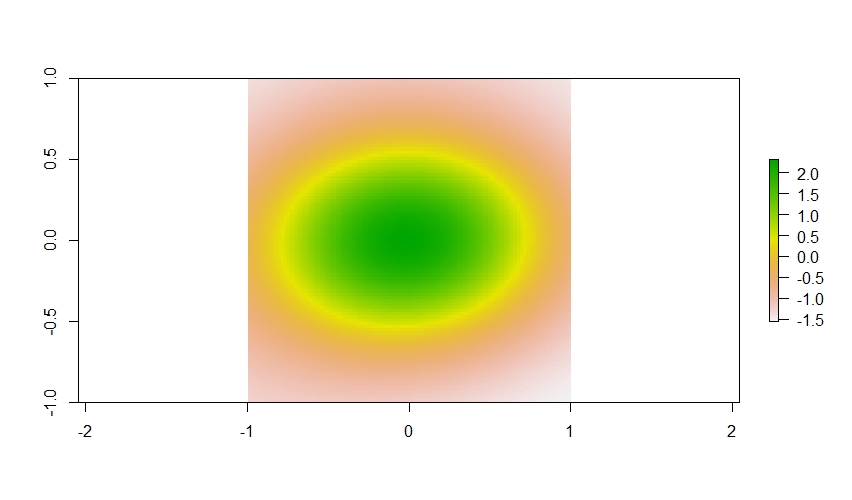
With these two covariates generated, we can go ahead and simulate some data. Let’s put some survey sites over the landscape, generate some species occupancy data there, and try to sample them imperfectly.
 # The number of survey sites.
nsite <- 250

# very rough and somewhat even spacing of sites on landscape
my_sites <- floor(
  seq(
    1, raster::ncell(plane), length.out = nsite
   )
)

# move half the sites a little bit so they don't end up in a straight line
jiggle_sites <- sort(
  sample(
    1:nsite, floor(nsite/2), replace = FALSE
  )
)

# add the jiggled sites back into my_sites
my_sites[jiggle_sites] <- floor(
  my_sites[jiggle_sites] + median(diff(my_sites)/2)
)

# This shuffling process could mean we have a value >
#   the number of cells in the raster. Fix it if this
#   is the case.
if(any(my_sites > raster::ncell(plane))){
  my_sites[my_sites > raster::ncell(plane)] <- raster::ncell(plane)
  my_sites <- unique(my_sites)
}
And here is where we are sampling across this landscape.
plot(plane$spatial)
points(xy[my_sites,], pch = 21, bg = "gray50")
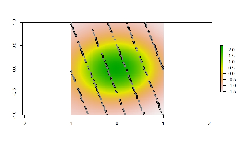
With the covariates and sites created, we can now simulate species occupancy on the landscape. To add an interesting nonlinear pattern, let’s make it so the species is not as likely to occur in the green dot in the center of the spatially autocorrelated data.
my_covars <- values(plane)[my_sites,]

# We are going to multiply the spatial term by -1 here so the
#  species is more likely to be outside the green circle (
#  (which are positive values). Additionally, let's say the
#  species is more likely to occur in areas of high forest cover.

# The occupancy parameters
sim_params <- c(-1, 0.5)

logit_prob <- my_covars %*% sim_params

species_prob <- plogis(logit_prob)

# Simulate occupancy on landscape

z <- rbinom(nsite, 1, species_prob)

# Plot it out
plot(plane$spatial)
points(xy[my_sites[z == 1],], pch = 21, bg = "blue")
points(xy[my_sites[z == 0],], pch = 21, bg = "grey50")
legend(
  "bottomleft",
  pt.bg = c("blue", "grey50"),
  legend =c("present", "absent"),
  pch = 21,
  bty = "n"
)
And here are the sites where this species does and does not occupy. Generally, this species is not found in that central circle on the landscape.
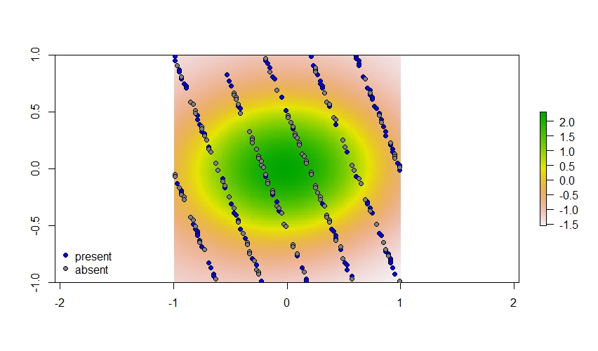
Finally, we get to add some refreshing realism to these data and make the ecologists who went out and collected these data make some mistakes (i.e., add imperfect detection). Nevertheless, we are going to assume they still did an adequate job sampling (i.e., above average detection probability) and that there is no spatial variation in detection.
# Detection probability
det_prob <- 0.4
# The number of repeat surveys
n_survey <- 4

# The simulated data we would have 'in hand' at the end of the study
y <- rbinom(
  nsite,
  n_survey,
  det_prob * z
)
Step 2. Create a Generalized Additive Occupancy Model
Okay, and now we can actually start doing some modeling! To create
the spatial smoothing term we can use mgcv::jagam(). We’re going
to use a thin plate smooth spline on the site coordinates in order
to capture the spatial correlation in this species occupancy pattern.
The mgcv::jagam() function essentially spins up a GAM in the JAGS
programming language. Therefore, all we need to do is pull out the essential
pieces of that JAGS script and add it to a standard Bayesian occupancy model. Aside
from specifying the type of smoother you want to fit, you also need
to input the number of basis functions to generate for the GAM. The higher the number, the slower the model fit, but you also want to make sure you add enough to be able to capture the non-linear complexity in the data (see ?mgcv::choose.k for more details on this). For this example, we are going to use 15. Finally, mgcv::jagam() also creates a few
data objects we need to pass to the model, so it’s important to assign the output to some variable.
# Get site coordinates
site_coords <- xy[my_sites,]

# The temporary GAM we will take apart.
tmp_jags <- mgcv::jagam(
  response ~ s(
    x, y, k = 15, bs = "ds", m = c(1,0.5)
    ),
  data = data.frame(
    response = rep(1, nsite),
    x = site_coords[,1],
    y = site_coords[,2]
  ),
  family = "binomial",
  file = "tmp.jags"

)
As we named the file tmp.jags you can open it up in R with file.edit(tmp.jags). It looks like this (below), which already comes with some helpful comments. Now, we could just modify this model to create an occupancy model, but I’m only going to pull out the necessary pieces and add it to a new jags script.
So, we start with this jags script:
model {
  eta <- X %*% b ## linear predictor
  for (i in 1:n) { mu[i] <-  ilogit(eta[i]) } ## expected response
  for (i in 1:n) { y[i] ~ dbin(mu[i],w[i]) } ## response
  ## Parametric effect priors CHECK tau=1/11^2 is appropriate!
  for (i in 1:1) { b[i] ~ dnorm(0,0.0083) }
  ## prior for s(x,y)...
  K1 <- S1[1:14,1:14] * lambda[1]
  b[2:15] ~ dmnorm(zero[2:15],K1)
  ## smoothing parameter priors CHECK...
  for (i in 1:1) {
    lambda[i] ~ dgamma(.05,.005)
    rho[i] <- log(lambda[i])
  }
}
Most everything we need is towards the bottom of the script. After removing some for loops we did not need and modifying some priors we end up with:
  ## Parametric effect priors
  b[1] ~ dnorm(0,0.75)
  ## prior for s(x,y)...
  K1 <- S1[1:14,1:14] * lambda[1]
  b[2:15] ~ dmnorm(zero[2:15],K1)
  ## smoothing parameter priors CHECK...
  lambda ~ dgamma(.05,.005)
  rho <- log(lambda)
Which can be thrown into a standard occupancy model.
model{
  for(i in 1:nsite){
    # Latent state, b is the smoothing term, beta_occ is the effect of forest cover.
    logit(psi[i]) <- inprod(b,X[i,]) + inprod(beta_occ,covs[i,])
    z[i] ~ dbern(psi[i])
    # Detection
    logit(det_prob[i]) <- beta_det
    y[i] ~ dbin(det_prob[i] * z[i], nsurvey)
  }
  # the priors
  beta_occ ~ dnorm(0, 0.75)
  beta_det ~ dnorm(0, 0.75)
  ## Parametric effect priors
  b[1] ~ dnorm(0,0.75)
  ## prior for s(x,y)...
  K1 <- S1[1:14,1:14] * lambda[1]
  b[2:15] ~ dmnorm(zero[2:15],K1)
  ## smoothing parameter priors...
  lambda ~ dgamma(.05,.005)
  rho <- log(lambda)
}
One important thing to note in this model is that the first b term in the spatial smoothing function is actually the model intercept. If you investigate the X matrix from tmp_jags via head(tmp_jags$jags.data$X) you’ll see the first column is all 1’s. Thus, that first b term represents the overall spatial average while the remaining terms indicate how that spatial average varies through space, while controlling for the influence of other covariates in the model (and of course assuming that you have centered and scaled the other covariates in the model).
Step 3. Fit the model
Assuming you save this model as a script (e.g., occupancy_gam.R), then you
can fit the model. There are a few bits from the mgcv::jagam call
that also need to be added (S1, X, and zero), so we add those to our
data list we supply to JAGS as well. The model does not especially sample
all that efficiently, so we are doing a relatively long model run (note: I would still likely run this longer if this was a real project, the effective sample size of some of the smoothing term regression coefficients is still quite low).
# data to include
data_list <- list(
  y = y,
  X = tmp_jags$jags.data$X,
  S1 = tmp_jags$jags.data$S1,
  covs = matrix(my_covars[,2], ncol = 1, nrow = nsite),
  nsite = nsite,
  nsurvey = n_survey,
  zero = tmp_jags$jags.data$zero
)

# initial values function
my_inits <- function(chain){
  gen_list <- function(chain = chain){
    list(
      z = rep(1, nsite),
      beta_occ = rnorm(1),
      beta_det = rnorm(1),
      b = rnorm(
      	length(tmp_jags$jags.ini$b),
      	tmp_jags$jags.ini$b,
      	0.2
      ),
      lambda = rgamma(1,1,1),
      .RNG.name = switch(chain,
        "1" = "base::Wichmann-Hill",
        "2" = "base::Wichmann-Hill",
        "3" = "base::Super-Duper",
        "4" = "base::Mersenne-Twister",
        "5" = "base::Wichmann-Hill",
        "6" = "base::Marsaglia-Multicarry",
        "7" = "base::Super-Duper",
        "8" = "base::Mersenne-Twister"
      ),
      .RNG.seed = sample(1:1e+06, 1)
		)
	}
	return(switch(chain,
		"1" = gen_list(chain),
		"2" = gen_list(chain),
		"3" = gen_list(chain),
		"4" = gen_list(chain),
		"5" = gen_list(chain),
		"6" = gen_list(chain),
		"7" = gen_list(chain),
		"8" = gen_list(chain)
	)
	)
}

# Long model run to increase effective sample size
my_mod <- runjags::run.jags(
  model = "occupancy_gam.R",
  monitor = c("b", "beta_occ", "beta_det", "rho"),
  inits = my_inits,
  data = data_list,
  n.chains = 3,
  adapt = 1000,
  burnin = 100000,
  sample = 20000,
  thin = 20,
  method = "parallel"
)

# summarize model
my_sum <- summary(my_mod)
Step 4. Check how well the model did
Because we have simulated data, we can actually see how well the smoothing term captured the spatial autocorrelation in our data. Now, our goal is for the model to estimate the simulated values in our spatially autocorrelated data. We used 15 basis functions to do this. What’s important to note here is that the individual regression coefficients for each of the b should not especially be interpreted on their own. Instead, it is the combined effect of all of them that create our spatial pattern. To check how well the model performs then, we can simply generate a model prediction for what each spatial value should be at each of our 250 survey sites and see if the true value is within the 95% credible interval of that estimate. I’m leaving out graphical model checking for the other parameters, but the true parameter values fell well within the 95% credible intervals for the effect of forest cover (true = 0.5, estimate = 0.63, 95% CI = 0.24, 1.05) and detection probability (true = -0.4, estimate = -0.5, 95% CI = -0.74, 0.26).
# Combine the three mcmc chains
my_mcmc <- do.call('rbind', my_mod$mcmc)

# Make the spatial prediction across all 250 sites for each
#  step in the MCMC chain, then calculate 95% credible interval.
spatial_est <- data_list$X %*% t(my_mcmc[,1:15])
spatial_est <- apply(
  spatial_est, 1, quantile, probs = c(0.025,0.5,0.975)
)

# Combine these estimates with the true values
#  Note: Multiplying the true values by -1 because that is how
#  we simualted the data.

spatial_est <- cbind(
  t(spatial_est), my_covars[,1] * -1
)
# order by the true values
spatial_est <- spatial_est[order(spatial_est[,4]),]

# Just a quick check to determine if true value in within
#   95% credible interval at all sites. It's TRUE.
sum(
  spatial_est[,4] > spatial_est[,1] &
  spatial_est[,4] < spatial_est[,3]
) == nsite

# Plot this out.
plot(
  spatial_est[,2] ~ c(1:nsite), ylim = range(hm), type = "n",
  bty = "l",
  xlab = "Sites",
  ylab = "Spatial value at each site"
)
for(i in 1:nsite){
  # Add 95% credible intervals
  lines(
    y = spatial_est[i,c(1,3)], x = rep(i,2)
  )
}
# Add the true values as well
points(spatial_est[,4], pch = 21, bg = "grey50")
In this plot, the vertical lines are 95% credible intervals for each survey site. The points represent the true
values we simulated in planes$spatial. The true values sit within the credible intervals for each site, so it
looks like we’ve done an okay job with capturing the spatial autocorrelation in these data.

However, in an actual analysis, you will not have simulated values for comparison. So how do you interpret your spatial smoothing term? One way is to plot it out.
# get the median estimate of the spatial smoothing term
#  which are the first 15 values in the model summary, column 2.
median_est <- data_list$X %*% my_sum[1:15,2]

# We already have the site coordinates, so we just need to
#  generate the colors we want to plot out.

# This is roughly the range of the model estimates
cuts <- seq(-2.1, 2.6, length.out = 255)

# Classify the median estimate into a color category
median_est_colors <- as.numeric(
  cut(median_est, cuts)
)

# And the colors (similar to other plots)
my_terrain <- terrain.colors(255)
plot(
  x = xy[my_sites,1],
  y = xy[my_sites,2],
  pch = 21,
  bg = my_terrain[median_est_colors],
  cex = 2,
  xlab = "x",
  ylab = "y",
  bty = "l"
)
And sure enough it looks like it does an okay job capturing the pattern.
We can take this one step further, however, and plot those simulated values over the landscape we generated.

And that is one way you you can make a generalized additive occupancy model in R!
Session info.
R version 4.0.3 (2020-10-10)
Platform: x86_64-w64-mingw32/x64 (64-bit)
Running under: Windows 10 x64 (build 19043)

Matrix products: default

locale:
[1] LC_COLLATE=English_United States.1252
[2] LC_CTYPE=English_United States.1252
[3] LC_MONETARY=English_United States.1252
[4] LC_NUMERIC=C
[5] LC_TIME=English_United States.1252

attached base packages:
[1] stats     graphics  grDevices utils     datasets
[6] methods   base

other attached packages:
[1] mvtnorm_1.1-0   raster_3.1-5    sp_1.4-2
[4] runjags_2.0.4-6 mgcv_1.8-33     nlme_3.1-149

loaded via a namespace (and not attached):
 [1] rstan_2.21.2         tidyselect_1.1.0
 [3] xfun_0.13            purrr_0.3.4
 [5] splines_4.0.3        lattice_0.20-41
 [7] generics_0.1.0       V8_3.3.1
 [9] colorspace_1.4-1     vctrs_0.3.7
[11] stats4_4.0.3         loo_2.3.1
[13] rlang_0.4.10         pkgbuild_1.0.8
[15] pillar_1.4.3         glue_1.4.0
[17] withr_2.2.0          matrixStats_0.56.0
[19] lifecycle_1.0.0      munsell_0.5.0
[21] gtable_0.3.0         codetools_0.2-16
[23] coda_0.19-3          inline_0.3.16
[25] knitr_1.28           callr_3.4.3
[27] ps_1.3.3             parallel_4.0.3
[29] curl_4.3             fansi_0.4.1
[31] Rcpp_1.0.4.6         scales_1.1.1
[33] RcppParallel_5.0.2   StanHeaders_2.21.0-6
[35] jsonlite_1.6.1       gridExtra_2.3
[37] ggplot2_3.3.0        processx_3.4.2
[39] dplyr_1.0.5          grid_4.0.3
[41] rgdal_1.5-8          cli_2.0.2
[43] tools_4.0.3          magrittr_1.5
[45] tibble_3.0.1         crayon_1.3.4
[47] pkgconfig_2.0.3      ellipsis_0.3.0
[49] Matrix_1.2-18        prettyunits_1.1.1
[51] assertthat_0.2.1     rstudioapi_0.11
[53] R6_2.4.1             compiler_4.0.3