A simple static occupancy model in NIMBLE
I have to be honest. It’s been a while since I’ve actually thought about fitting a static, or single season, occupancy model. Why? The lab I am part of has been camera trapping in Chicago for over a decade. So naturally, we generally use different classes of occupancy models with our data. Yet, while I may not use this model, other researchers certainly do! Likewise, if you want to understand more complicated occupancy models, it makes sense to get a decent grasp of some of the earliest models.
So if you are just getting into occupancy modeling and need a gentle introduction, look no further! However, before jumping into this, I would be remiss to not point out that there are a LOAD of wonderful resources that provide a much more thorough explanation then I will here. Some that come to mind are MacKenzie et al. (2017) or Volume 1 of Applied Hierarchical Modeling in Ecology by Kéry and Royle.
After providing a brief motivating example, I’ll show four separate static occupancy models. Without getting ahead of myself, there are a few different ways to write these models out, and which one you choose to use will depend on your study design and research goals.
A motivating example
When we go out and try to determine if a species occupies an area of interest, we end up with ‘false-absences’ in our observed data in the event that a species occupies an area and we fail to detect it. For this example, let’s assume we have 100 locations we are sampling and the true probability of occupancy for our species of interest is 0.75. If we wanted to simulate such data in R we could do something like:
# True Pr(occupancy) on landscape
occ_prob <- 0.75

# simulate latent occupancy 1000 times at 100 sites
nsite <- 100
nsim <- 1000

# fill matrix column-wise, 100 sites per simulation
z <- matrix(
  rbinom(
    nsite * nsim,
    1,
    occ_prob
  ),
  nrow = nsite,
  ncol = nsim
)

# plot out the variability in latent occupancy
# across the 1000 simulations
hist(
  colMeans(z),
  main = "",
  xlab = "Occupancy probability"
)
# add true occupancy
abline(v = occ_prob, lty = 2, lwd = 3)
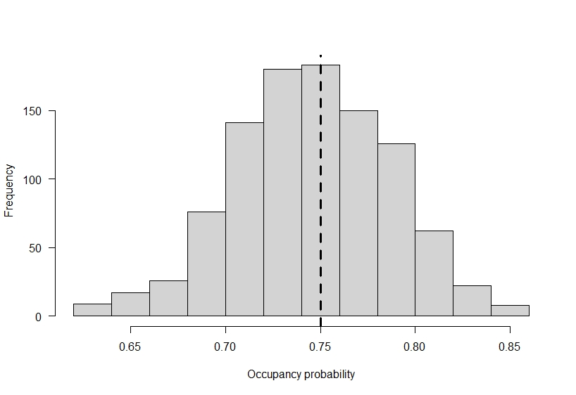
If ecologists had the power of a Disney princess and all the animals of the forest would line up and say hello, we would perfectly observe the occupancy status of our species of interest at each site. It would be great, and modeling could simply be done with logistic regression. However, ecologists are fallible. We make mistakes, and species can be present at a location and go undetected. To continue our example, lets assume we only have a 0.35 probability of detecting a species if it is present. If we only visit each site one time, the observed occupancy we find at the end of our study is going to be substantially lower then the true occupancy on the landscape based on the way we set up this example.
# Add in observational error
det_prob <- 0.35

# simulate "observed" data. If z == 1, then we detect
#   the species with Pr(0.35) and y == 1, otherwise it
#   is 0.
y <- matrix(
  rbinom(
    nsite * nsim,
    1,
    z * det_prob
  ),
  nrow = nsite,
  ncol = nsim
)


# plot out the variability in observed occupancy
# across the 1000 simulations
hist(
  colMeans(y),
  main = "",
  xlab = "Observed occupancy probability",
  las = 1
)
# add in expected observed occupancy
abline(v = occ_prob * det_prob, lty = 2, lwd = 3)
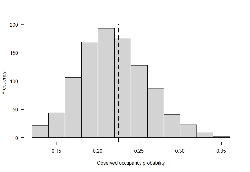
In reality, occupancy is 0.75, but our observed data suggests it is much lower! Of course, the example I used here is meant to show a large difference. If you do not detect species perfectly on the landscape, then going out to a site only once can add more false-absences, or zeroes, in your data then you’d expect based on a species distribution.
Occupancy models are meant to help with this, but they do not do so for ‘free.’ In fact, to separately estimate species occupancy and detectability they require repeat visits to sites under a time frame that you expect species occupancy to be constant. By revisiting sites, you can generate repeated observations of the detection process. This makes it possible to create a ‘capture history’ at each site, which can be represented as a series of 1’s and 0’s to reflect times a species was and was not detected on a repeat visit. If we were just going to simulate some data once (instead of 1000 times as above), this could look something like:
set.seed(444)
# latent occupancy prob
occ_prob <- 0.75

# detection probability
det_prob <- 0.35

# number of sites
nsite <- 100

# number of visits
J <- 5

# simulate latent occupancy
z <- rbinom(
  nsite,
  1,
  occ_prob
)

# simulate a capture history for each site.
#  We need to repeat each element of z  J
#  times to do this. Filling in row-wise
#  so that this matrix is nsite by nvisits
y <- matrix(
  rbinom(
    nsite * J,
    1,
    rep(z, each = J) * det_prob
  ),
  ncol = J,
  nrow = nsite,
  byrow = TRUE
)

# see if species is present at first 5 sites
head(z)
[1] 1 1 1 1 1 1


# look at first few capture histories
head(y)

      [,1] [,2] [,3] [,4] [,5]
[1,]    0    0    0    0    0
[2,]    0    1    1    0    0
[3,]    1    0    0    0    1
[4,]    0    1    0    1    1
[5,]    1    0    0    0    0
[6,]    1    0    0    0    0
With five revisits to each location, we have five opportunities to detect the species. If the species is present over the five surveys, then we sometimes detect it and sometimes do not (e.g., the second row above). Other times, even if it is present we miss it all five times (e.g., the first row above). And even other times, the species is not present at a site, and then it is impossible to detect it there, assuming that you do not falsely recognize some other species as your target species.
With the simulated data above, we are going to fit a static occupancy model in NIMBLE. Following this, we’ll expand the model a bit so we can include covariates on occupancy and detection.
An oldie but a goodie, the static occupancy model
Let \(\Psi\) be the probability of occupancy and z be a Bernoulli random variable that equals 1 if a the species is present and 0 if it is absent. For i in 1,…,I site the probability of occupancy is:
\[z_{i} \sim Bernoulli(\Psi)\]Let \(\rho\) be the conditional probability of detection. Thus, for j in 1,…,J repeat surveys let \(y_{i,j}\) be the observed data, which equals 1 if the species was detected and is otherwise 0. The observation model is then:
\[y_{i,j} \sim Bernoulli(\rho \times z_{i})\]Conversely, if we assume that each of the J revisits are independent and identically distributed (you often see this written as i.i.d.), then we could just use the Binomial distribution instead of independent Bernoulli trials. For modeling, this could be helpful as it could dramatically speed up your run times, but it would not be possible if there are observation level covariates that vary across visits (e.g., a different observer goes out across visits, precipitation, etc.). If this assumption holds with your own data, then you let \(r_{i}\) be the number of times the species was detected across J surveys (i.e,. the row sum of the Y matrix) and
\[r_{i} \sim Binomial(J, \rho \times z_{i})\]Following this, we need to add a parameter model to our Bayesian analysis. As we are modeling everything on the probability scale we will assume vague and uninformative priors for \(\Psi\) and \(\rho\) such that:
\[\Psi \sim Beta(1,1)\] \[\rho \sim Beta(1,1)\]which is essentially a uniform distribution between 0 and 1.
Given the data we generated above, the two detection models I presented are equivalent. Let’s write them both out in NIMBLE.
Model 1: a static occupancy model with independent Bernoulli trials at the observation level
To be honest, it takes more code to simulate these data then it does to write it out in NIMBLE. To fit the model to the data we simulated above we need to write out the model using NIMBLE’s syntax and then prepare all the necessary objects to supply to the model. To do this we’ll load the nimble package, as well as MCMCvis, which provides some excellent model summary tools.
library(nimble)
library(MCMCvis)

# a static occupancy model in 13 lines of code!
occ_1 <- nimble::nimbleCode({
  # latent state and data models, in that order
  for(i in 1:nsite){
    z[i] ~ dbern(psi)
    for(j in 1:nvisit){
      y[i,j]  ~ dbern(z[i] * rho)
    }
  }
  # parameter models
  psi ~ dbeta(1,1)
  rho ~ dbeta(1,1)
}
)

# set up function for initial values,
# including latent state
my_inits <- function(){
  list(
    psi = rbeta(1,1,1),
    rho = rbeta(1,1,1),
    z = rep(1, nsite)
  )
}

# set up constant list
my_constants <- list(
  nsite = nsite,
  nvisit = J
)

# and data list
my_data <- list(
  y = y
)

# fit the model
model_1 <- nimble::nimbleMCMC(
  occ_1,
  constants = my_constants,
  data = my_data,
  inits = my_inits,
  monitors = c("psi", "rho"),
  niter = 15000,
  nburnin = 7500,
  nchains = 2
)

# look at the model summary
MCMCvis::MCMCsummary(
  model_1,
  digits= 2
)

    mean    sd 2.5%  50% 97.5% Rhat n.eff
psi 0.82 0.055 0.71 0.82  0.92    1  2852
rho 0.36 0.029 0.30 0.36  0.42    1  1827
As a reminder, we set \(\Psi = 0.75\) and \(\rho = 0.35\), which both fall within the 95% credible intervals of this model. So in general, it looks like we did a decent job estimating species occupancy and detectability!
Model 2: a static occupancy model with a Binomial at the observation level
Again, this model is almost completely identical, we mostly just need to summarize the data in a slightly different way. In fact, the model estimates are essentially identical!
occ_2 <- nimbleCode({
  # latent state and data models, in that order
  for(i in 1:nsite){
    z[i] ~ dbern(psi)
    r[i]  ~ dbin(z[i] * rho, nvisit)
  }
  # parameter models
  psi ~ dbeta(1,1)
  rho ~ dbeta(1,1)
}
)

# set up function for initial values,
# including latent state
my_inits <- function(){
  list(
    psi = rbeta(1,1,1),
    rho = rbeta(1,1,1),
    z = rep(1, nsite)
  )
}

# set up constant list
my_constants <- list(
  nsite = nsite,
  nvisit = J
)

# and data list, taking rowSums of y matrix
my_data <- list(
  r = rowSums(y)
)

# fit the model
model_2 <- nimble::nimbleMCMC(
  occ_2,
  constants = my_constants,
  data = my_data,
  inits = my_inits,
  monitors = c("psi", "rho"),
  niter = 15000,
  nburnin = 7500,
  nchains = 2
)

# look at model output
MCMCvis::MCMCsummary(
  model_2,
  digits= 2
)

    mean    sd 2.5%  50% 97.5% Rhat n.eff
psi 0.82 0.056 0.71 0.82  0.92    1  2832
rho 0.36 0.030 0.30 0.36  0.42    1  1840
In my own research I almost always use the second model with camera trap data. The reason for this is that repeat observation ‘days’ for a camera are essentially equivalent, so there is little to no need to use the independent Bernoulli parameterization.
Adding covariates
Extending this model out to incorporate covariates is not a difficult thing, you just need to apply the appropriate link functions to \(\Psi\) and \(\rho\). In this case, we’ll use the logit link. To recognize the fact that \(\Psi\) now varies spatially, we’ll add the site subscript to it. The latent state model then becomes:
\[logit(\Psi_{i,}) = \pmb{\beta}\pmb{x}_i\] \[z_{i} \sim Bernoulli(\Psi_{i})\]where \(\pmb{\beta}\pmb{x}_i\) represents a vector of regression coefficients (including the model intercept) and their associated covariates. As I’m using matrix notation for the linear predictor, I may have lost some people. In the above example, if we assume that we have one covariate in the model, we could also write it like this:
\[logit(\Psi_{i,}) = \beta_0 \times 1 + \beta_1 \times x_i\]where \(\beta_0\) is the intercept for the latent state model and \(\beta_2\) is the slope term. In the former representation the first element of the \(\pmb{x}_i\) is a 1 (to indicate that the model intercept is always included). We could simplify this secondary representation even further if we wanted to so that it becomes:
\[logit(\Psi_{i,}) = \beta_0 + \beta_1 \times x_i\]Anyways, the latent state model can now incorporate covariates. Let’s do the same thing for the observation model. If we had observation level covariates, then we would need to use the independent Bernoulli parameterization for this level of the model:
\[logit(\rho_{i,j}) = \pmb{\alpha}\pmb{w}_{i,j}\] \[y_{i,j} \sim Bernoulli(\rho_{i,j} \times z_{i})\]where \(\pmb{\alpha}\pmb{w}_{i,j}\) represents a vector of regression coefficients for the observation model and their associated covariates (that vary at each site and survey).
If we did not have covariates that change over surveys then we could use the Binomial parameterization instead. The detection model would then be:
\[logit(\rho_{i}) = \pmb{\alpha}\pmb{w}_{i}\] \[r_{i} \sim Binomial(J, \rho_{i} \times z_{i})\]Finally, we need to add the parameter model. For logit scale coefficients, a standard choice for a vague prior would be to use Logistic(0,1) distributions, which converts back to a uniform distribution on the probability scale.
Let’s simulate some data under both models with covariates and fit them in nimble.
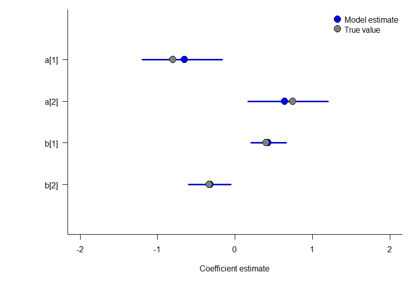
Model 3: a static occupancy model with covariates and independent Bernoulli trials at the observation level
Simulating the observation level model can be a little difficult to do (it’d be easier to read if I used more for loops / less matrix math to do so). Regardless, here is some simulated data to demonstrate this model, and we compare the results at the end to the parameters that simulated the data.
# number of sites and visits
set.seed(54)
nsite <- 100
nvisit <- 5
# latent state regression coefficients, logit scale
b <- c(0.75, -0.8)
# latent state covariates
x <- cbind(
1, rnorm(nsite)
)
# logit scale occupancy
psi_logit <- x %*% b
# convert to probability
psi_prob <- plogis(
psi_logit
)
# sample latent state
z <- rbinom(
nsite,
1,
psi_prob
)
# observation level regression coefficients, logit scale
a <- c(-0.33, 0.4)
# observation covariates, varies by visit so making
# this an array. Making array first filled with all
# 1's
w <- array(
1,
dim = c(
length(a),
nsite,
nvisit
)
)
# put a covariate in w[2,,]
w[2,,] <- rnorm(
nsite * nvisit
)
# fill in logit scale detection probability with for loop
det_logit <- matrix(
NA,
ncol = nvisit,
nrow = nsite
)
for(j in 1:nvisit){
det_logit[,j] <- t(w[,,j]) %*% a
}
# convert to a probability
det_prob <- plogis(det_logit)
# we now have a separate probablity of detection for every visit.
# Let's simulate the observed data now. This code is a little
# confusing here because of:
# rep(z, each = nvisit) * as.numeric(t(det_prob))
# Basically, it replicates we element of z nvisit times and
# multiplies it by the correct element in det_prob. To get the
# correct element in det_prob, we transpose it so its dimensions
# become nvisit by nsite and then convert it to a numeric.
y <- matrix(
rbinom(
nsite * nvisit,
1,
rep(z, each = nvisit) * as.numeric(t(det_prob))
),
ncol = nvisit,
nrow = nsite,
byrow = TRUE
)
# write nimble model
occ_3 <- nimbleCode({
# latent state and data models, in that order
for(i in 1:nsite){
logit(psi[i]) <- inprod(
b[1:npar_psi],
x[i,1:npar_psi]
)
z[i] ~ dbern(psi[i])
for(j in 1:nvisit){
logit(rho[i,j]) <- inprod(
a[1:npar_rho],
w[1:npar_rho, i, j]
)
y[i,j] ~ dbern(z[i] * rho[i,j])
}
}
# parameter models
for(psii in 1:npar_psi){
b[psii] ~ dlogis(0,1)
}
for(rhoi in 1:npar_rho){
a[rhoi] ~ dlogis(0,1)
}
}
)
# set up function for initial values,
# including latent state
my_inits <- function(){
list(
b = rnorm(2),
a = rnorm(2),
z = rep(1, nsite)
)
}
# set up constant list
my_constants <- list(
nsite = nsite,
nvisit = nvisit,
npar_psi = ncol(x),
npar_rho = dim(w)[1]
)
# and data list
my_data <- list(
y = y,
x = x,
w = w
)
# fit the model
model_3 <- nimble::nimbleMCMC(
occ_3,
constants = my_constants,
data = my_data,
inits = my_inits,
monitors = c("b", "a"),
niter = 15000,
nburnin = 7500,
nchains = 2
)
model_3_results <- MCMCvis::MCMCsummary(
model_3,
digits= 2
)
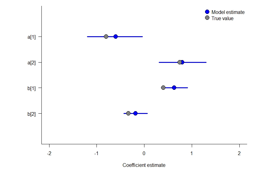
# and plot them out
par(mar = c(5,7,1,1))
plot(1~1, xlim = c(-2,2), ylim = c(0,5), type = "n", bty = "l",
xlab = "Coefficient estimate",
ylab = "", yaxt = "n")
axis(2, rev(1:4), row.names(model_3_results), las = 2)
for(i in 1:4){
# add 95% CI and median
lines(
x = c(
model_3_results[i,3],
model_3_results[i,5]
),
y = rep(i,2),
col = "blue",
lwd = 3
)
points(
x = median(model_3_results[i,4]),
y = i,
pch = 21,
bg = "blue",
cex = 2
)
}
points(c(b,a),y = c(3,4,1,2), pch = 21, bg = "gray50", cex = 2)
legend(
"topright",
c("Model estimate", "True value"),
pch = 21,
pt.bg = c("blue", "gray50"),
pt.cex = 2,
bty = "n"
)
Model 4: a static occupancy model with covariates an Binomial at the observation level
This model is much simpler to simulate. Again, given the sample size we have here and the small number of parameters it does a good job estimating the true values that simulated the data.
# number of sites and visits
set.seed(75)
nsite <- 100
nvisit <- 5

# latent state regression coefficients, logit scale
b <- c(0.75, -0.8)

# latent state covariates
x <- cbind(
  1, rnorm(nsite)
)

# logit scale occupancy
psi_logit <- x %*% b

# convert to probability
psi_prob <- plogis(
  psi_logit
)

# sample latent state
z <- rbinom(
  nsite,
  1,
  psi_prob
)

# observation level regression coefficients, logit scale
a <- c(-0.33, 0.4)

# observation covariates that do not vary by visit
w <- cbind(
  1,
  rnorm(nsite)
)


# fill in logit scale detection probability w
det_logit <- w %*% a


# convert to a probability
det_prob <- plogis(det_logit)

# fill in y matrix

y <- matrix(
  rbinom(
    nsite * nvisit,
    1,
    rep(z, each = nvisit) * rep(det_prob, each = nvisit)
  ),
  ncol = nvisit,
  nrow = nsite,
  byrow = TRUE
)

# write nimble model

occ_4 <- nimbleCode({
  # latent state and data models, in that order
  for(i in 1:nsite){
    logit(psi[i]) <- inprod(
      b[1:npar_psi],
      x[i,1:npar_psi]
    )
    z[i] ~ dbern(psi[i])
    logit(rho[i]) <- inprod(
      a[1:npar_rho],
      w[i, 1:npar_rho]
    )
    r[i]  ~ dbin(z[i] * rho[i], nvisit)
  }
  # parameter models
  for(psii in 1:npar_psi){
    b[psii] ~ dlogis(0,1)
  }
  for(rhoi in 1:npar_rho){
    a[rhoi] ~ dlogis(0,1)
  }
}
)

# set up function for initial values,
# including latent state
my_inits <- function(){
  list(
    b = rnorm(2),
    a = rnorm(2),
    z = rep(1, nsite)
  )
}

# set up constant list
my_constants <- list(
  nsite = nsite,
  nvisit = nvisit,
  npar_psi = ncol(x),
  npar_rho = ncol(w)
)

# and data list
my_data <- list(
  r = rowSums(y),
  x = x,
  w = w
)

# fit the model
model_4 <- nimble::nimbleMCMC(
  occ_4,
  constants = my_constants,
  data = my_data,
  inits = my_inits,
  monitors = c("b", "a"),
  niter = 15000,
  nburnin = 7500,
  nchains = 2
)


model_4_results <- MCMCvis::MCMCsummary(
  model_4,
  digits= 2
)

# and plot them out

par(mar = c(5,7,1,1))
plot(1~1, xlim = c(-2,2), ylim = c(0,5), type = "n", bty = "l",
     xlab = "Coefficient estimate",
     ylab = "", yaxt = "n")
axis(2, rev(1:4), row.names(model_4_results), las = 2)
for(i in 1:4){
  # add 95% CI and median
  lines(
    x = c(
      model_4_results[i,3],
      model_4_results[i,5]
    ),
    y = rep(i,2),
    col = "blue",
    lwd = 3
  )
  points(
    x = median(model_4_results[i,4]),
    y = i,
    pch = 21,
    bg = "blue",
    cex = 2
  )

}
points(c(b,a),y = c(3,4,1,2), pch = 21, bg = "gray50", cex = 2)

legend(
  "topright",
  c("Model estimate", "True value"),
  pch = 21,
  pt.bg = c("blue", "gray50"),
  pt.cex = 2,
  bty = "n"
)